Updates:
- 2023/02/09: finally published
- 2023/02/08: worked on text and illustrations a lot, many sample prints, multiple visualization approaches, details on f1 + f2 vs f1 * f2 and cylindrical and spherical transformation of TMPS
- 2023/01/05: adding mesh/voxel renderings, slicing geometry to generate G-code
- 2022/12/11: first FDM G-code generated using 2D / contour approach
- 2022/12/07: included many suitable periodic minimal surfaces
- 2022/12/02: start with implicit surface focus
As I progress I will update this blog-post.
Introduction
Infill geometries are geometries which are continuous, repetitive or periodic; they fill a boundary defined geometry aka outer form often defined via meshs. Let’s dive into some of the simple geometries and then looking at some more complex structures:
The Implicit Geometries
Implicit geometries are geometries defined via f(x,y,z) = 0 defining their surface, the boundary between inside and outside and they are ideal to define repetitive or periodic 3D infill geometries.
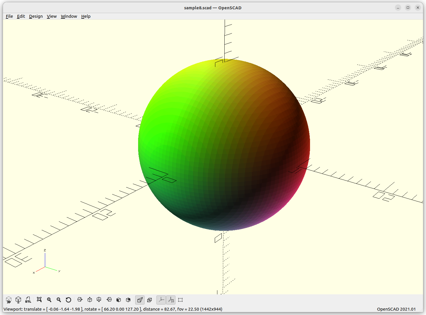
Sphere
Sphere: x2 + y2 + z2 – r2 = 0


When you ever tried to compose a sphere as a mesh, you know there are many ways to do so, and all are more complex than this simple description, and as you realize, the formula is perfect, it’s not an approximation – this is the nature of implicit formula. When you try to visualize an implicit formula, then you need to discretize and there the approximation takes place, as a mesh or as voxels.
Another nifty property of the sphere, it is the minimal surface to circumvent a volume, and through this blog-post, the minimal surface will become a common theme.
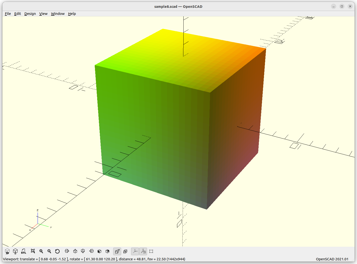
Cube
Cube: max(abs(x),abs(y),abs(z)) – w/2 = 0
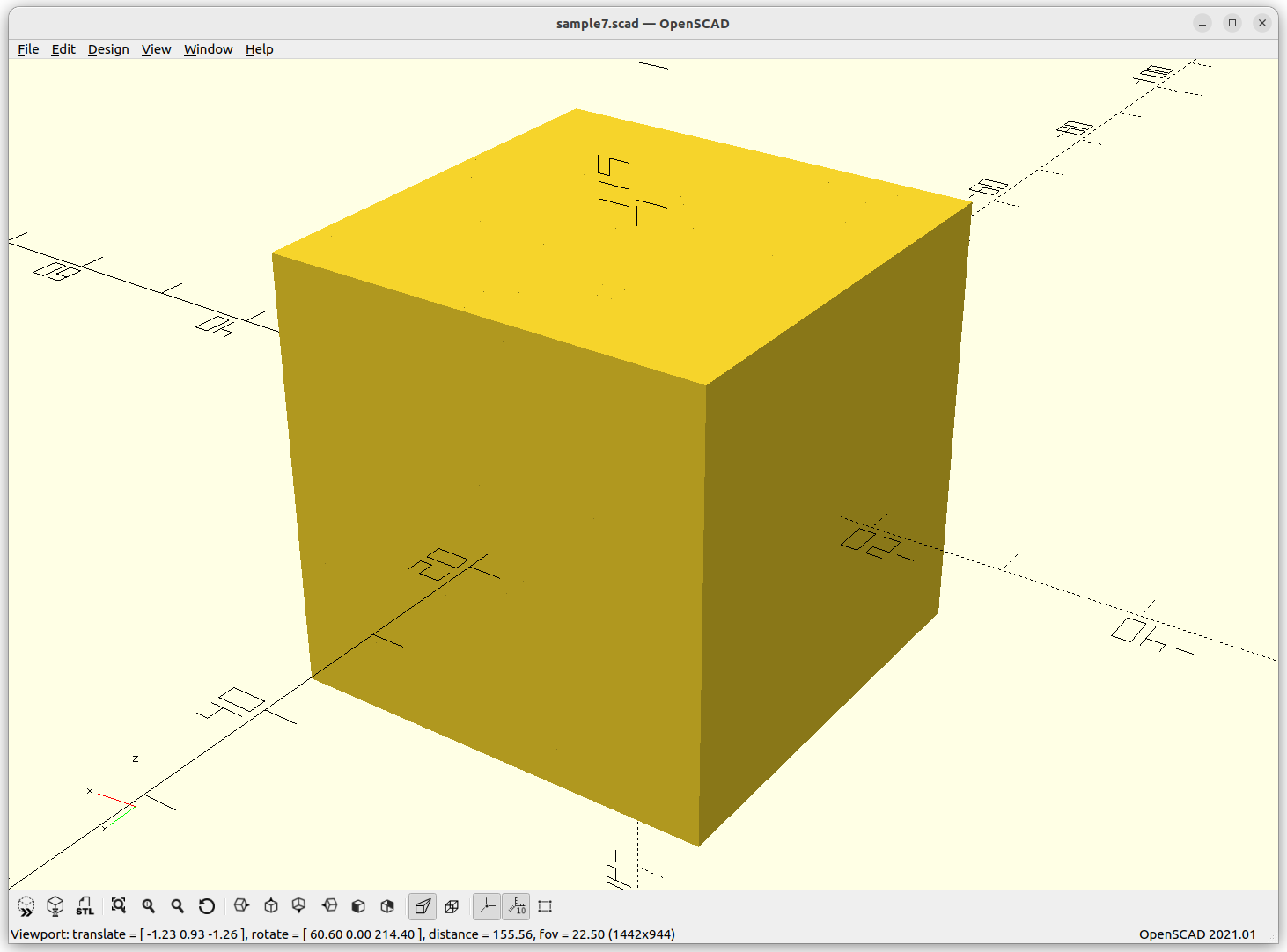
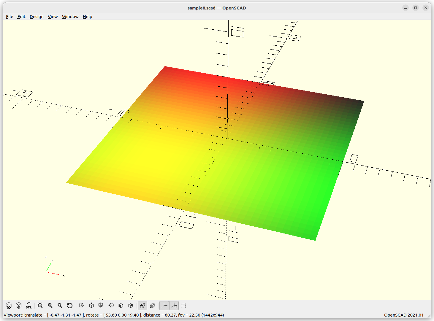
Plane
Plane: z = 0
As I render only -10 to 10 to each axis, it creates a small plate:

Triply Periodic Minimal Surface (TPMS)
Let’s move to the world of minimal surfaces, so called Triply Periodic Minimal Surfaces (TPMS), those can be expressed in implicit form and have some properties as sought for infill geometries.
In differential geometry, a triply periodic minimal surface (TPMS) is a minimal surface in ℝ3 that is invariant under a rank-3 lattice of translations. These surfaces have the symmetries of a crystallographic group. Numerous examples are known with cubic, tetragonal, rhombohedral, and orthorhombic symmetries. Monoclinic and triclinic examples are certain to exist, but have proven hard to parametrise.
Wikipedia: Triply Periodic Minimal Surface (TPMS), retrieved 2023/02/08
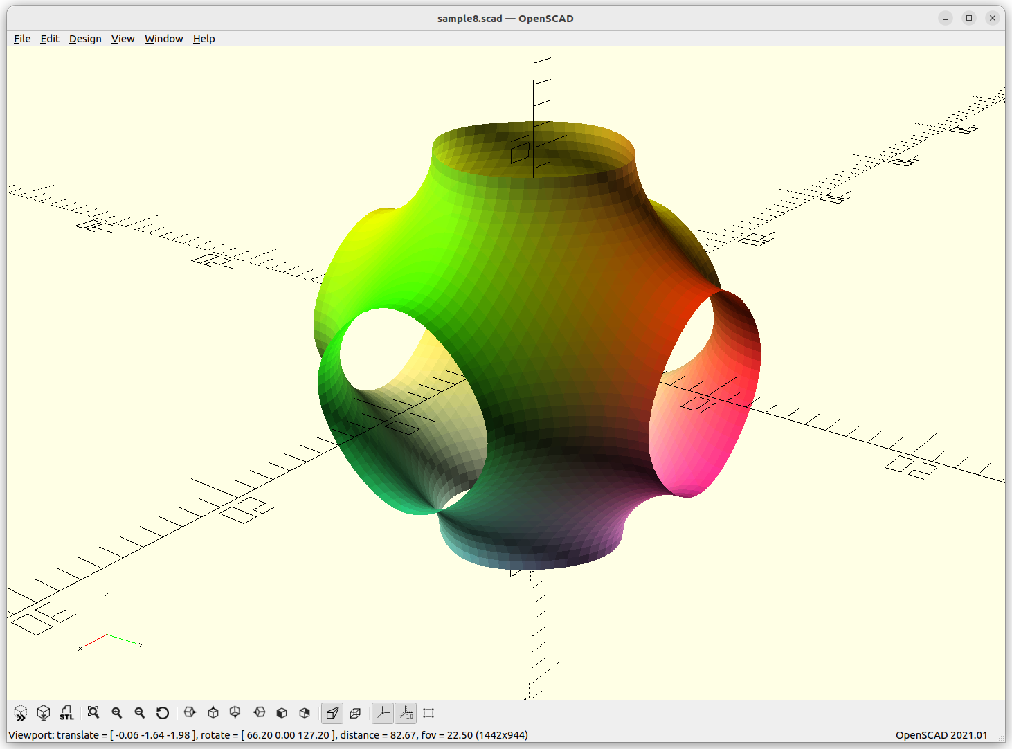
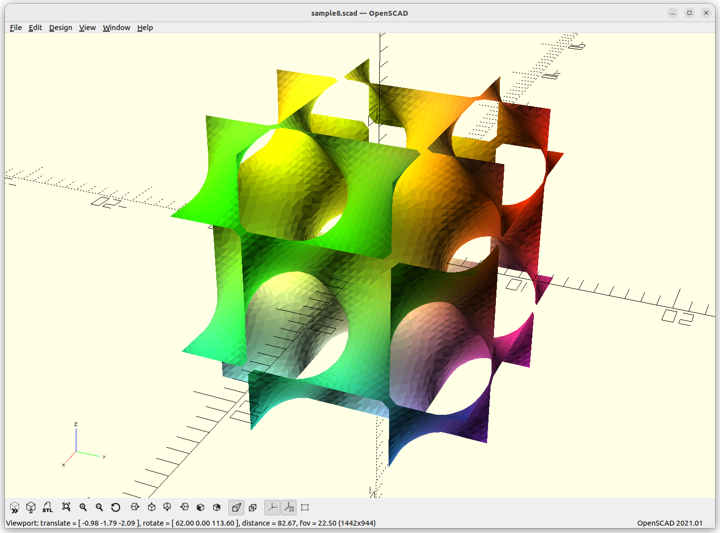
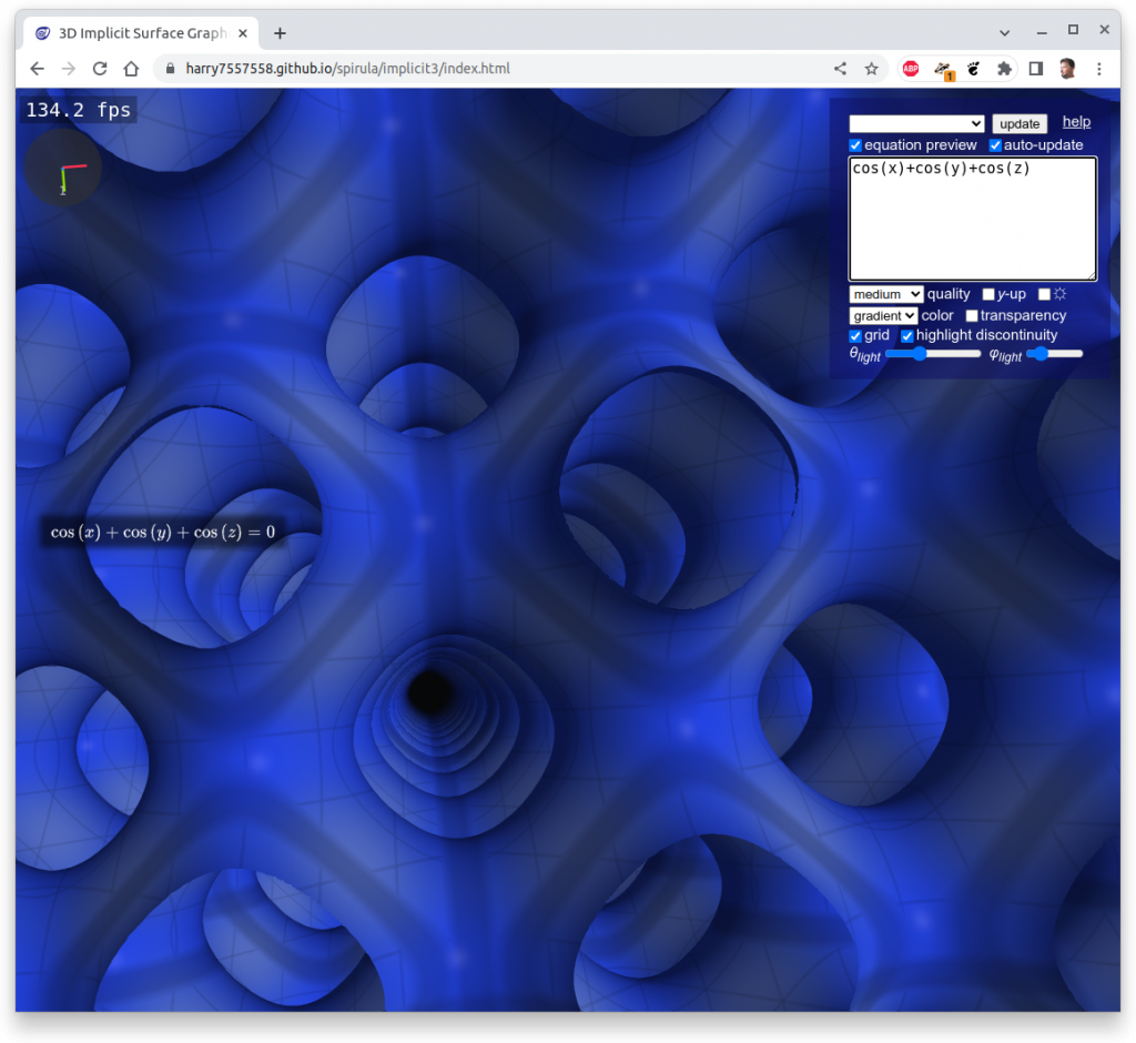
Schwarz P aka Primitive
One of the simplest yet powerful formula:
Schwarz P: cos(x) + cos(y) + cos(z) = 0
increasing the frequency or scale of the structure:
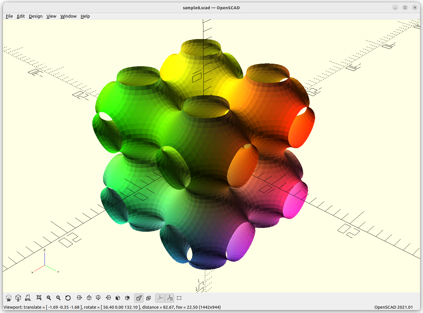

By extending the formula with +a, we can animate it:
Schwarz D aka Diamond
Schwarz D: sin(x)*sin(y)*sin(z) + sin(x)*cos(y)*cos(z) +
cos(x)*sin(y)*cos(z) + cos(x)*cos(y)*sin(z) = 0

Neovius
Neovius: 3*(cos(x)+cos(y)+cos(z)) + 4*cos(x)*cos(y)*cos(z) = 0

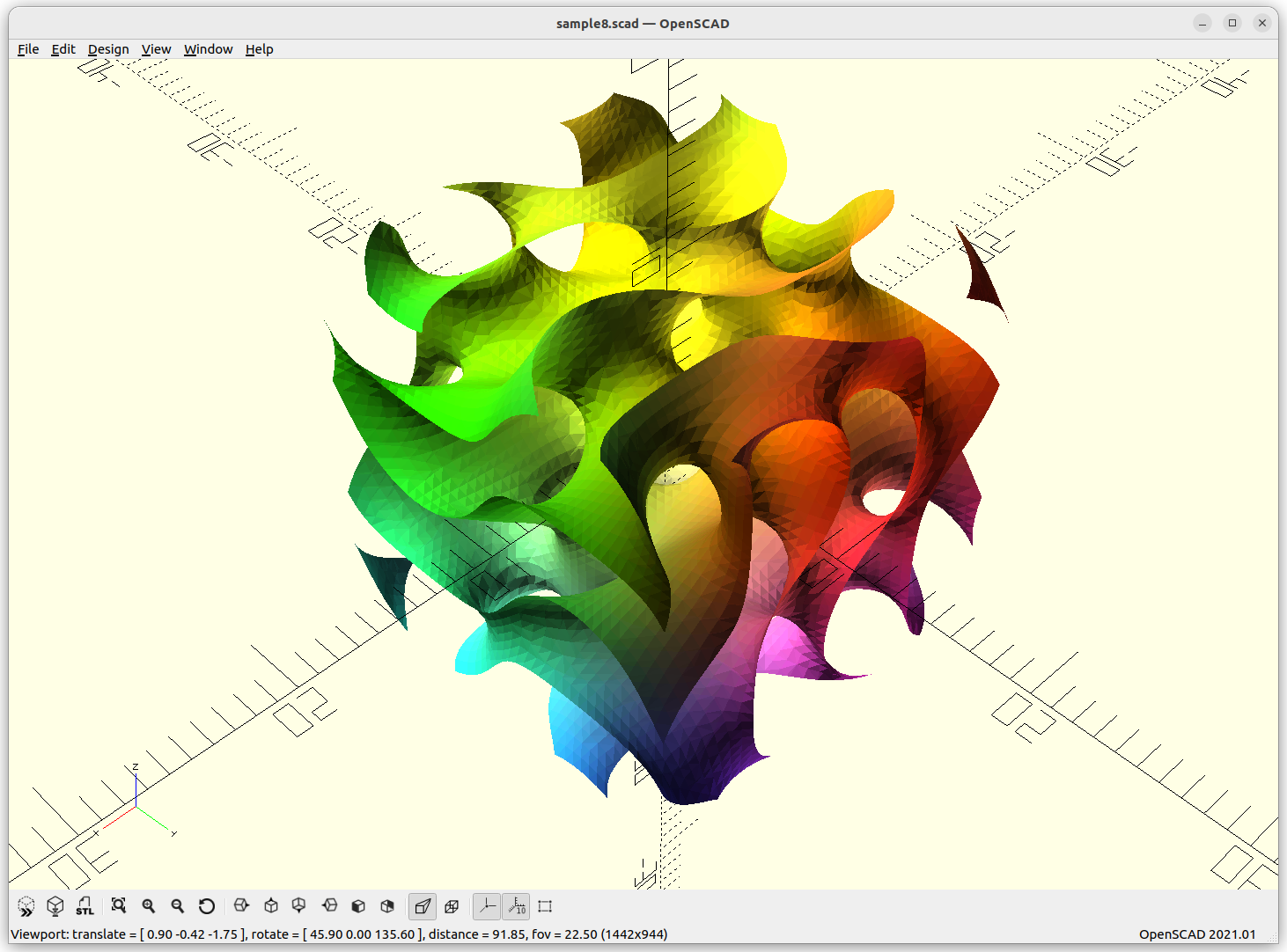
C(Y) Surface
C(Y) Surface: sin(x)*sin(y)*sin(z) + sin(2x)*sin(y) + cos(x)*sin(2y) + sin(2y)*sin(z) + sin(2z)*sin(x) + cos(x)*cos(y)*cos(z) + sin(2x)*cos(z) + cos(x)*sin(2y) + cos(y)*sin(2z) = 0

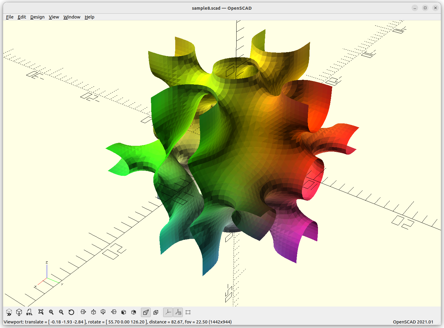
Fischer Koch
Fischer Koch: (cos(x)*cos(y)*cos(z) + cos(z)*cos(x)) –
(cos(2x)+cos(2y)+cos(2z)) = 0

S Surface
S Surface: cos(2x)*sin(y)*cos(z) + cos(2y)*sin(z)*cos(x) +
cos(2z)*sin(y)*cos(y) – 0.4 = 0

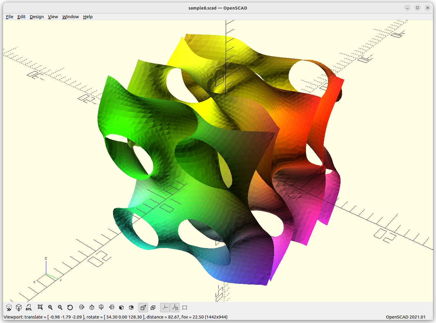
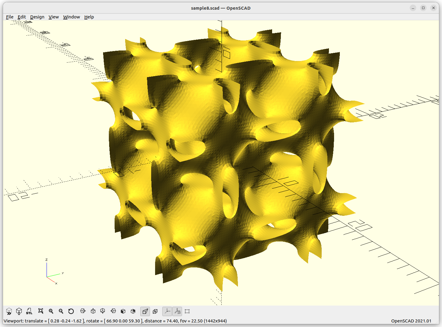
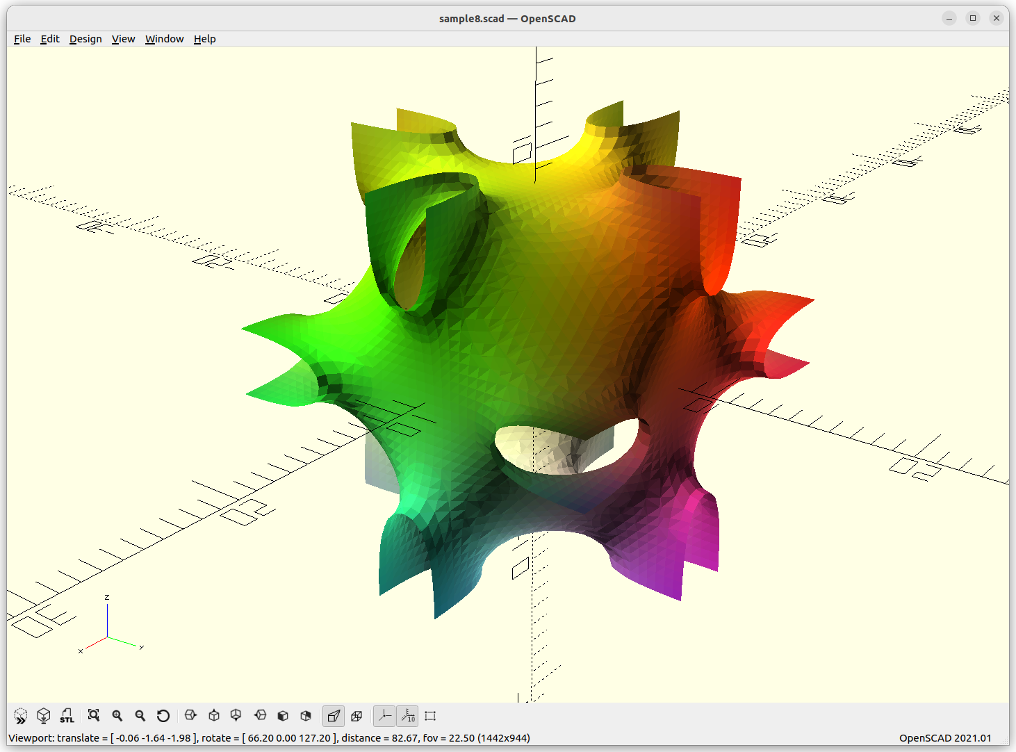
Gyroid
Gyroid: cos(x)*sin(y) + cos(y)*sin(z) + cos(z)*sin(x) = 0
FRD
FRD: 8 * a*cos(x)*cos(y)*cos(z) + b*(cos(2x)*cos(2y)*cos(2z)) –
c*cos(2x)*cos(2y) – d*cos(2y)*cos(2z) – e*cos(2z)*cos(2x)
Let’s explore this form more thoroughly, we animate a, b, c, d, and e and see what it does, essentially we animate -1 to 1 in sinus, 0 eliminates of the chunk of the formula:
Gyroid Skeletal
Gyroid Skeletal: 10*cos(x)*sin(y)+cos(y)*sin(z)+cos(z)*sin(x)) –
0.5*(cos(2x)*cos(2y)+cos(2y)*cos(2z)+cos(2z)*cos(2x)) – 14

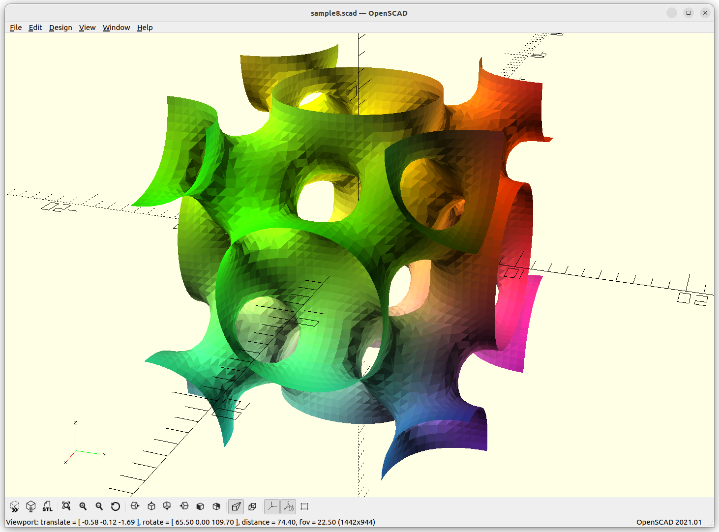
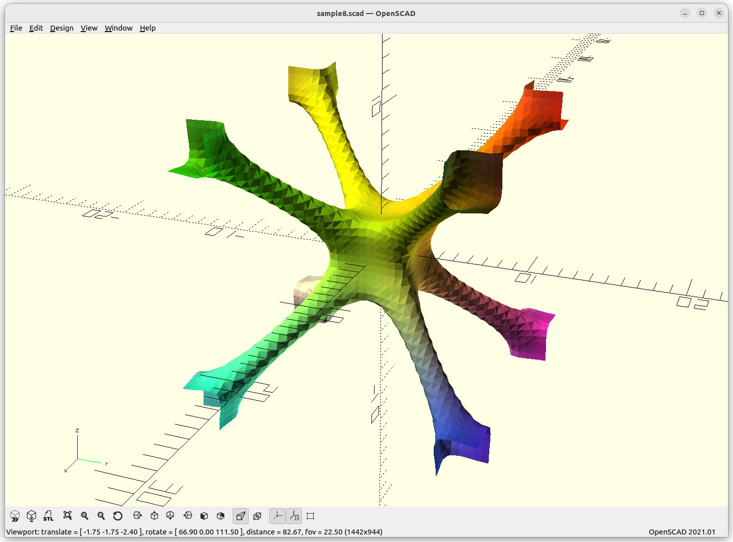
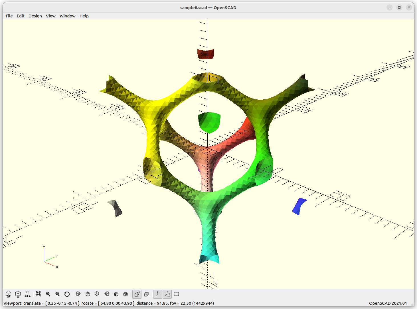
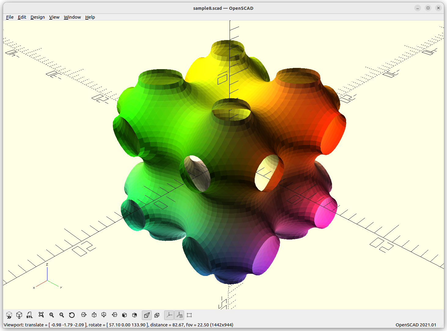
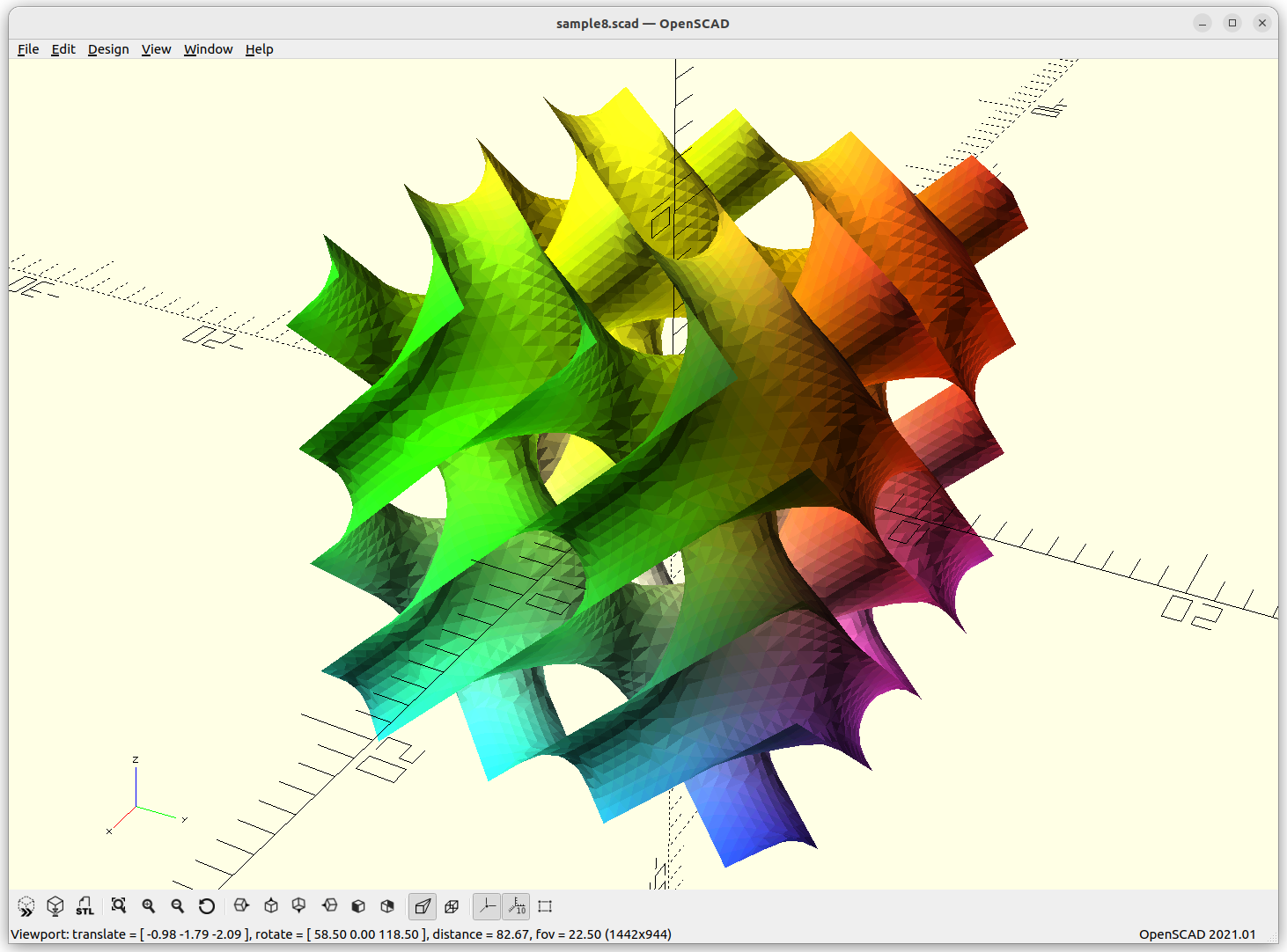
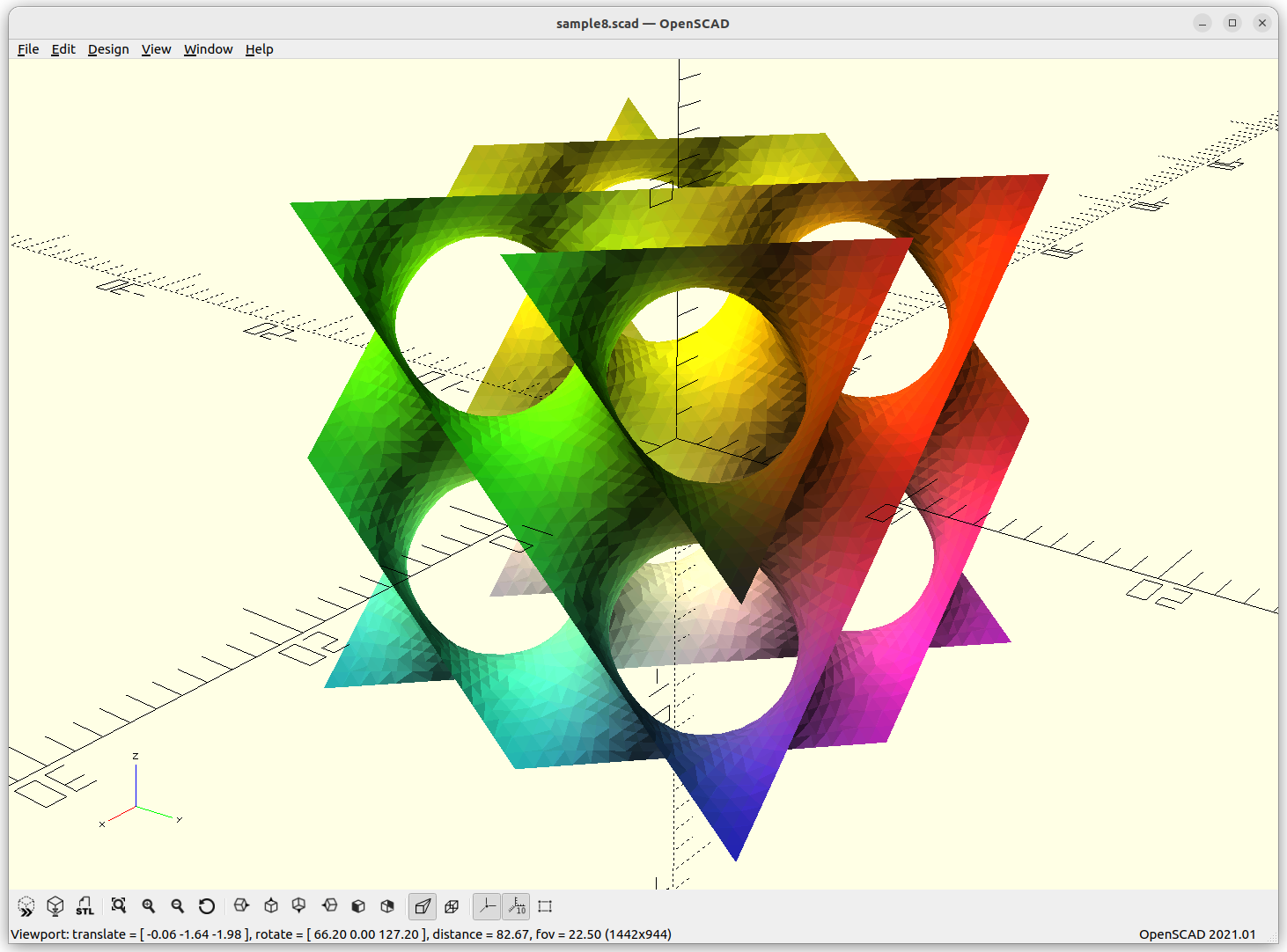
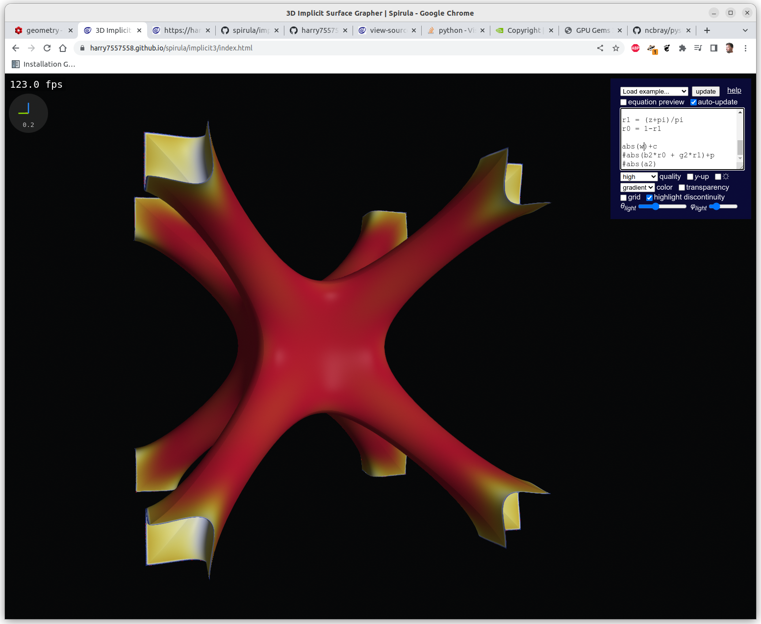
P Skeletal
P Skeletal: 10*(cos(x)+cos(y)+cos(z) –
5.1*(cos(x)*cos(y)+cos(y)*cos(z)+cos(z)*cos(x)) – 14.6
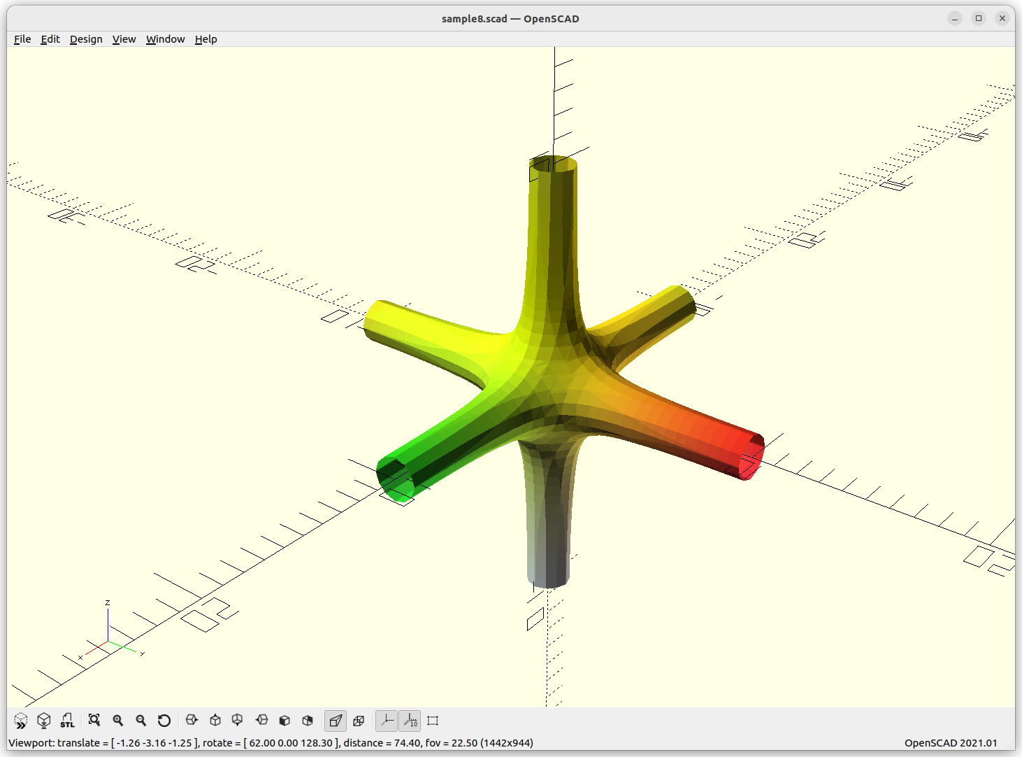
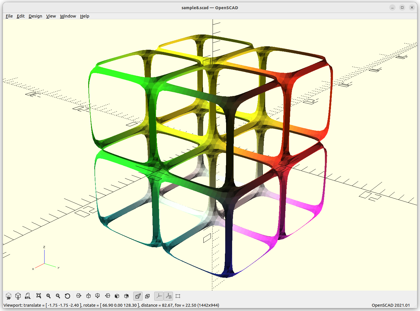


By changing the last substraction of 14.6 to 10 or 8, the structure get more dense – ideal to use.
The P Skeletal connects 6 arms to each other.
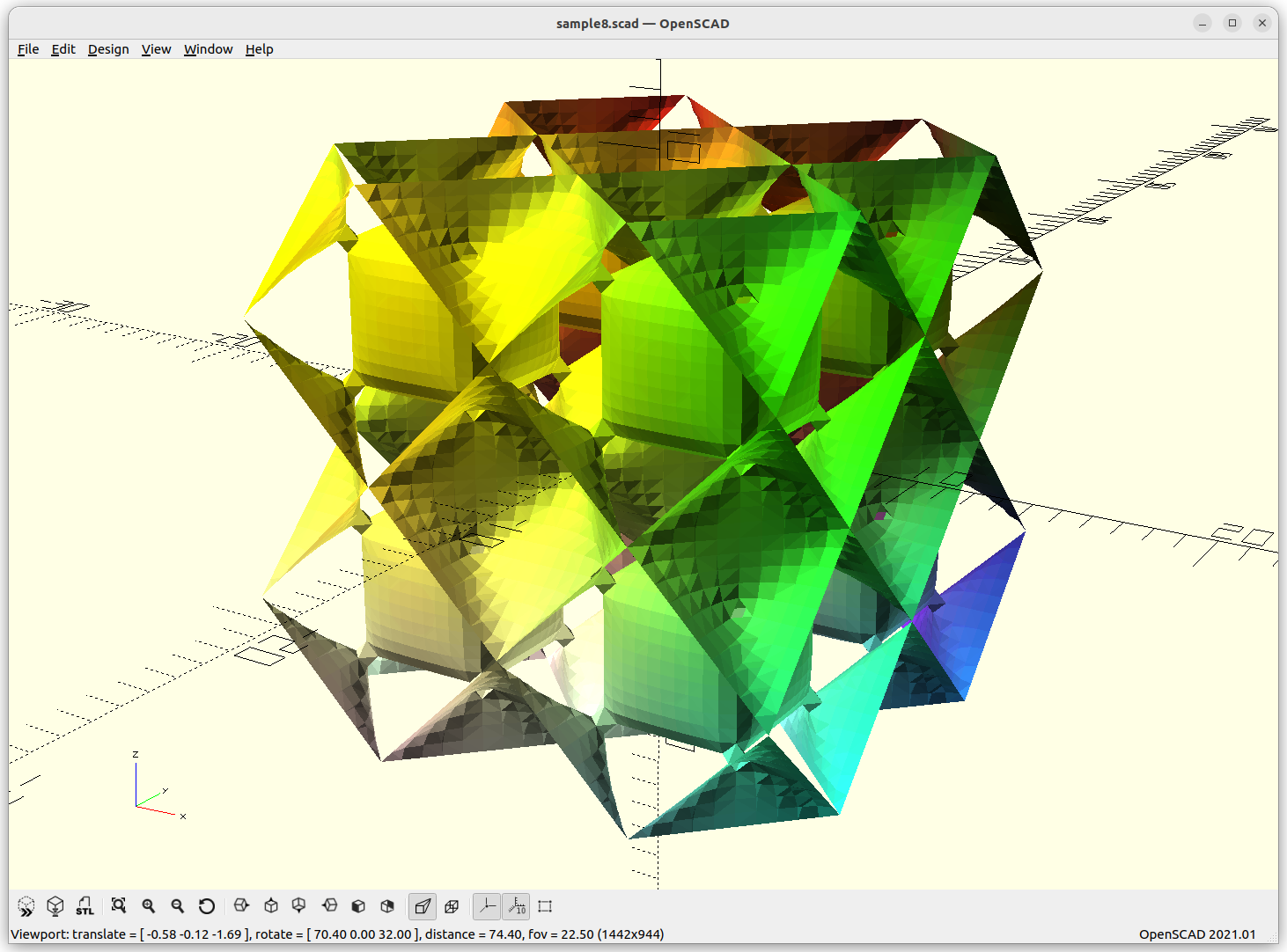
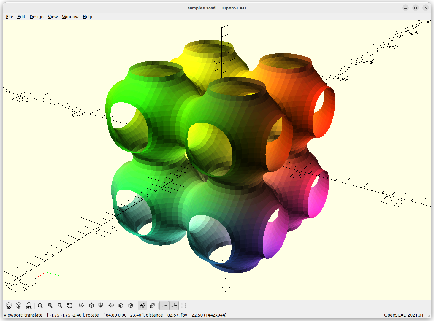
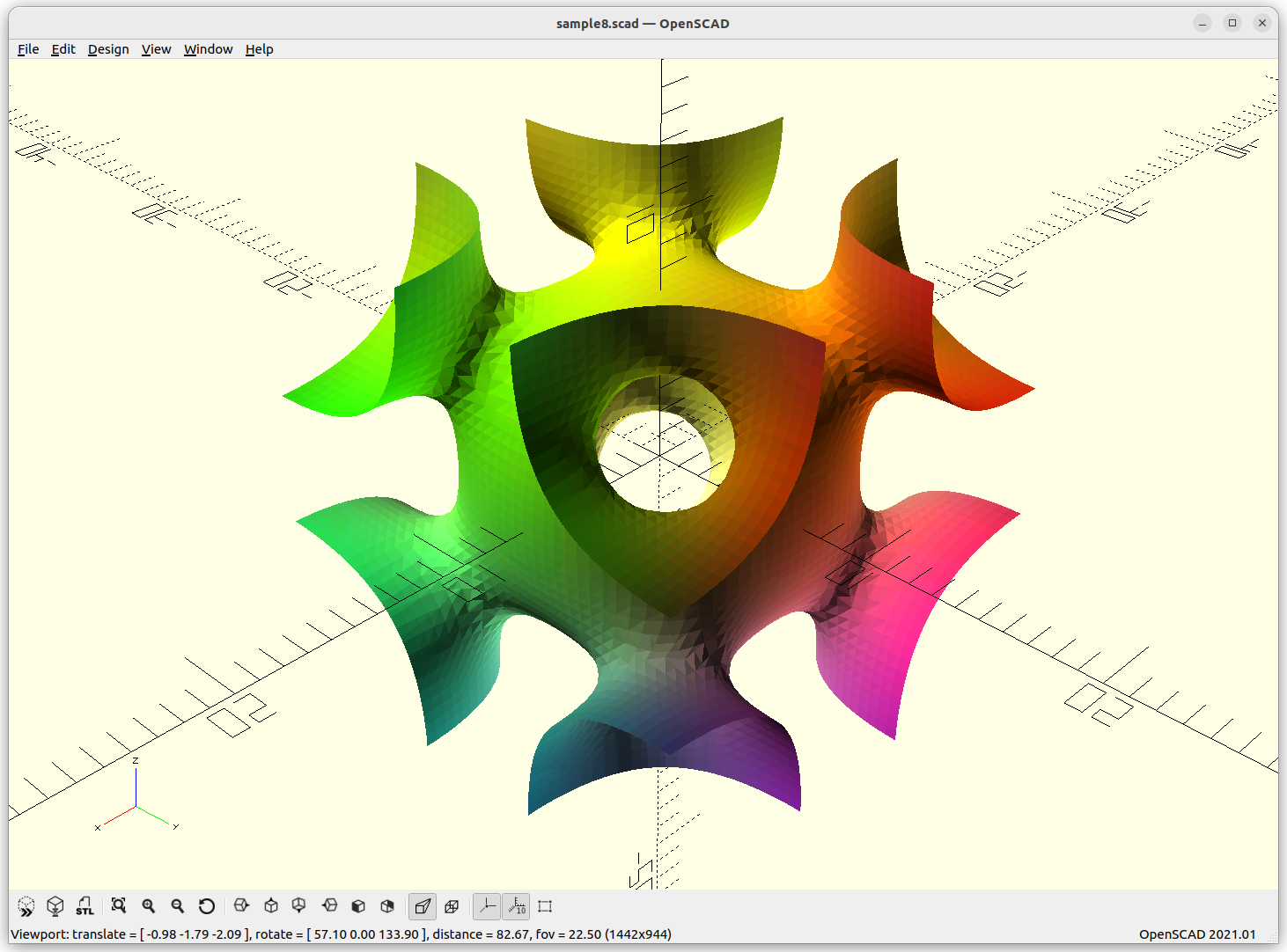
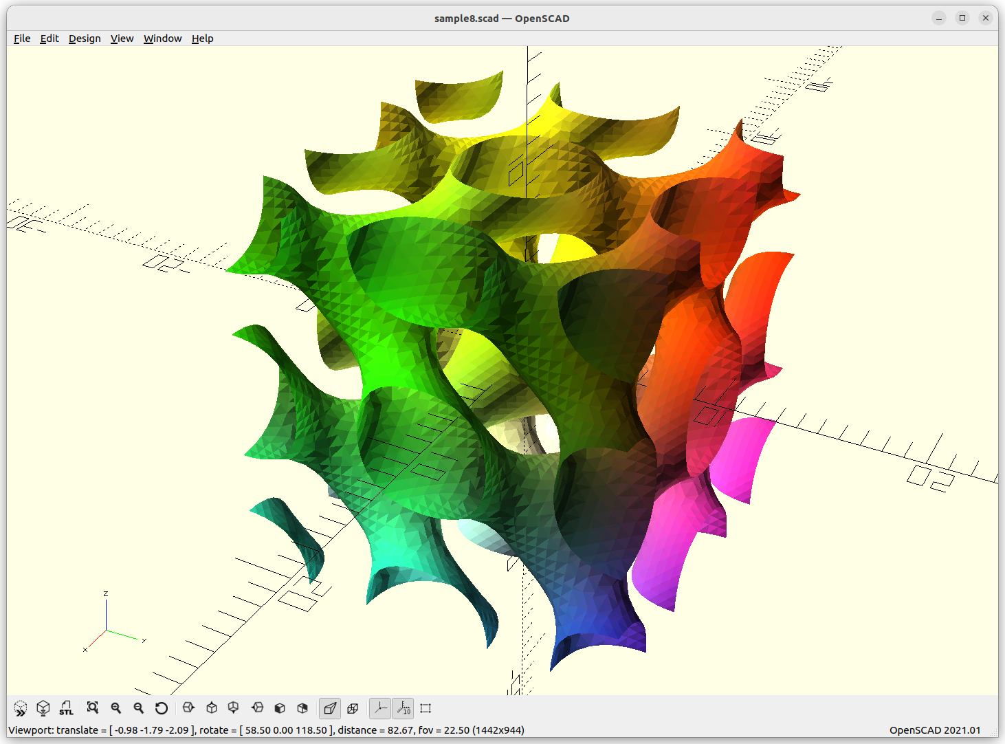
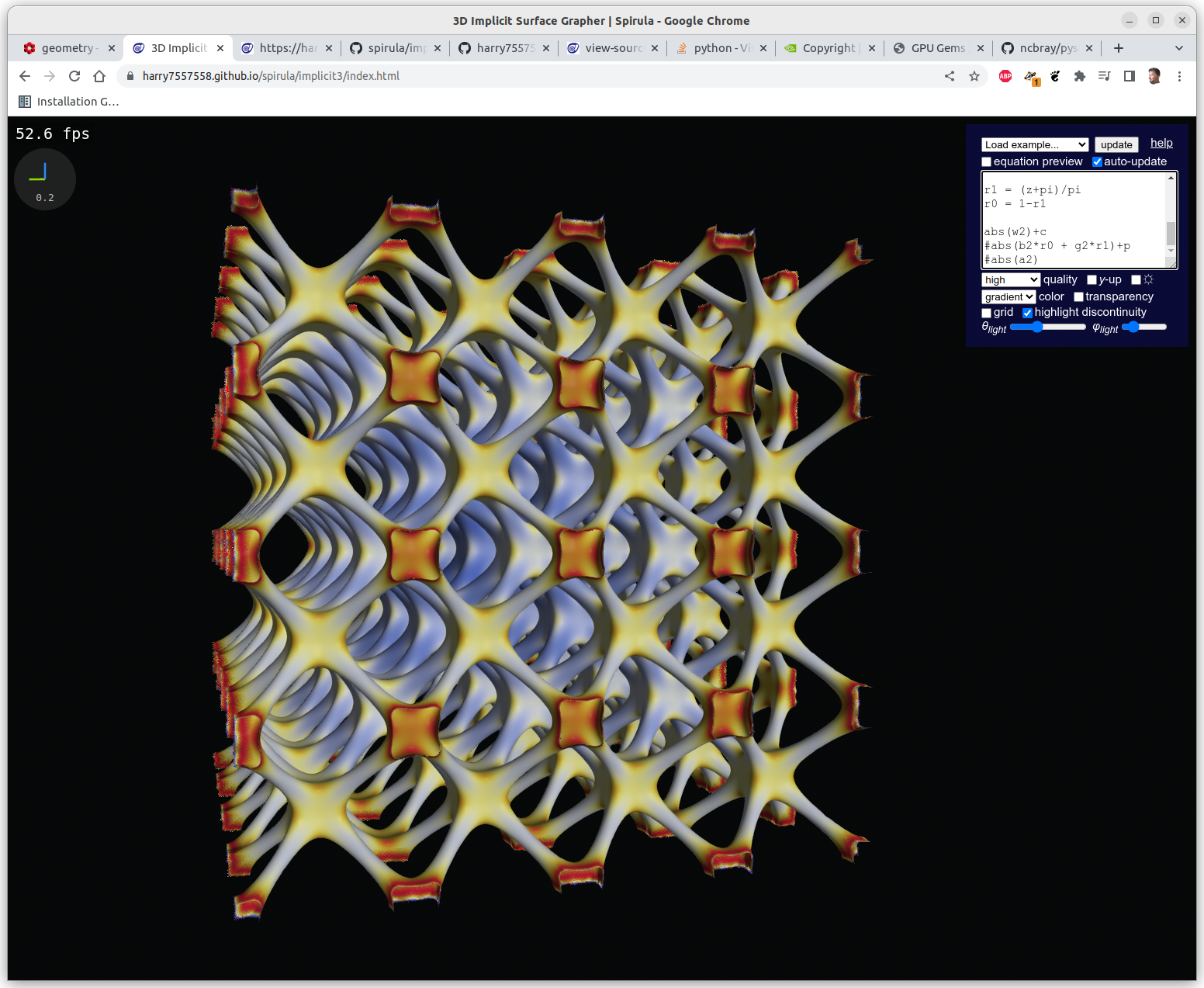
IWP Skeletal
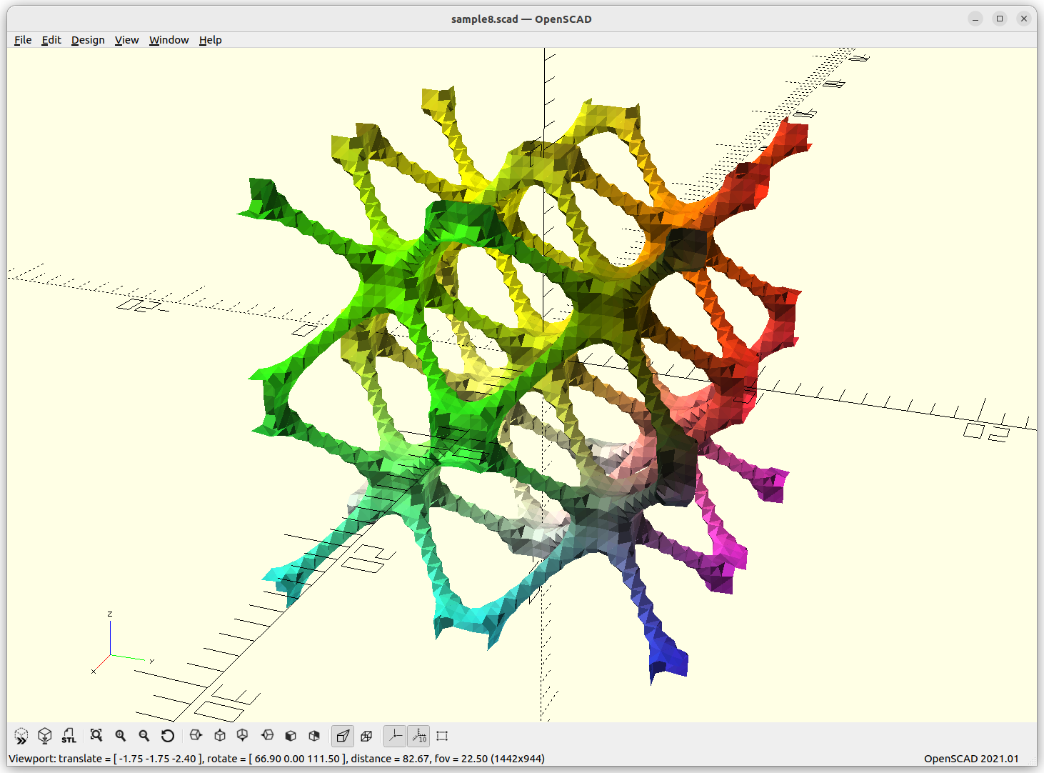
IWP Skeletal connects 8 arms to each other.
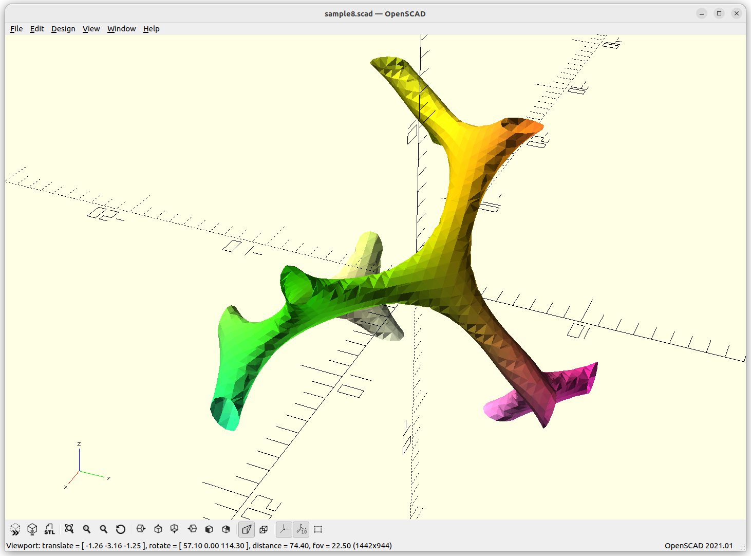
Schwarz D Skeletal

Schwarz D Skeletal connects with 4 arms to each other.
The above “skeletal” minimal surfaces are ideal for lattice structures, likely most usable in context of voxel-based 3D printing approaches, such as SLA, SLS, SLM and so forth, but less ideal for traditional FDM where the lattice is sliced Z-planar again kind of defeating the overall purpose of lattice structures.
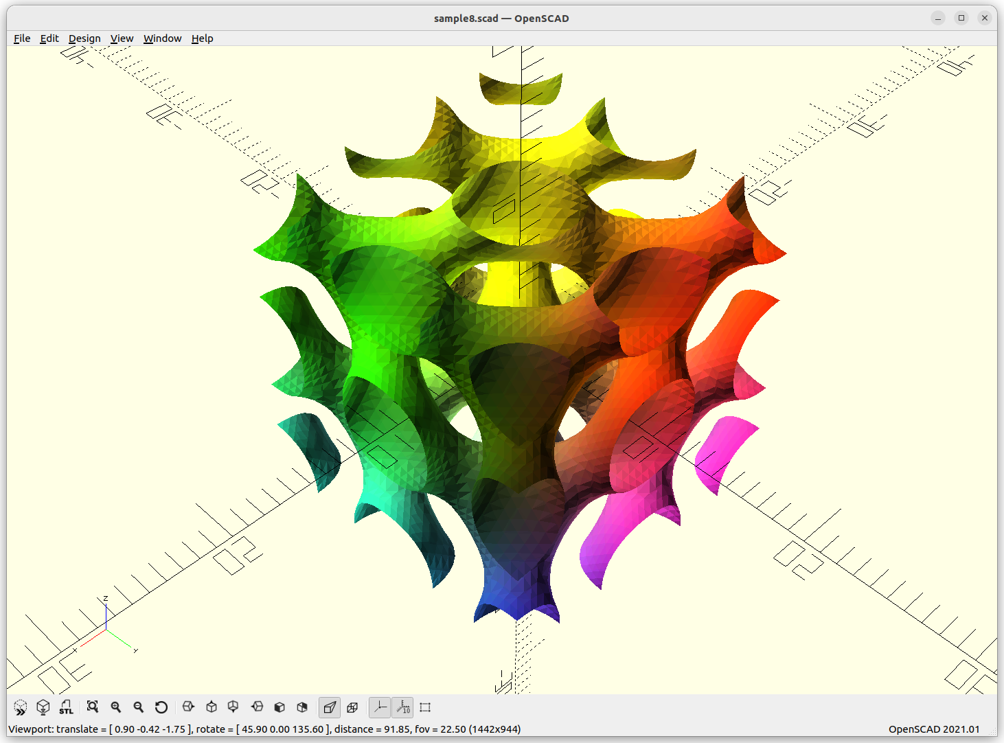
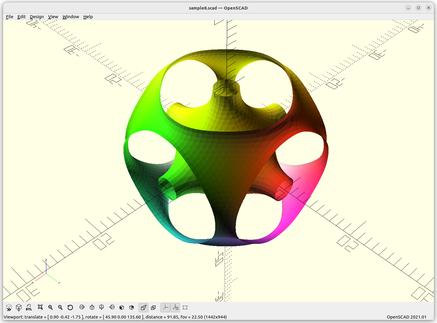
D Surface
D Surface: cos(x)*cos(y)*cos(z) – sin(x)*sin(y)*sin(z)
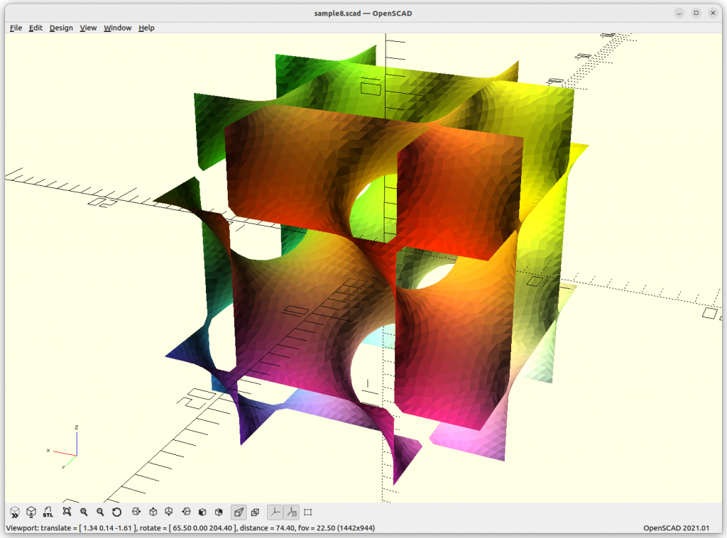
As Juergen Meier created a variant, adding a, which gives these variants:
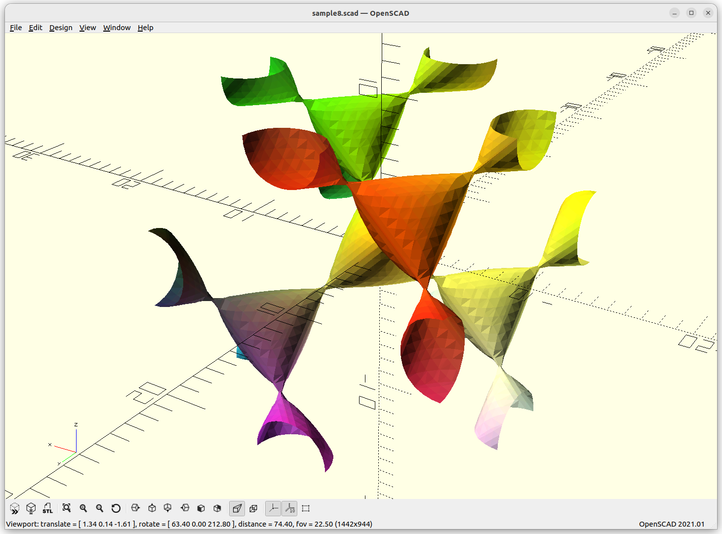
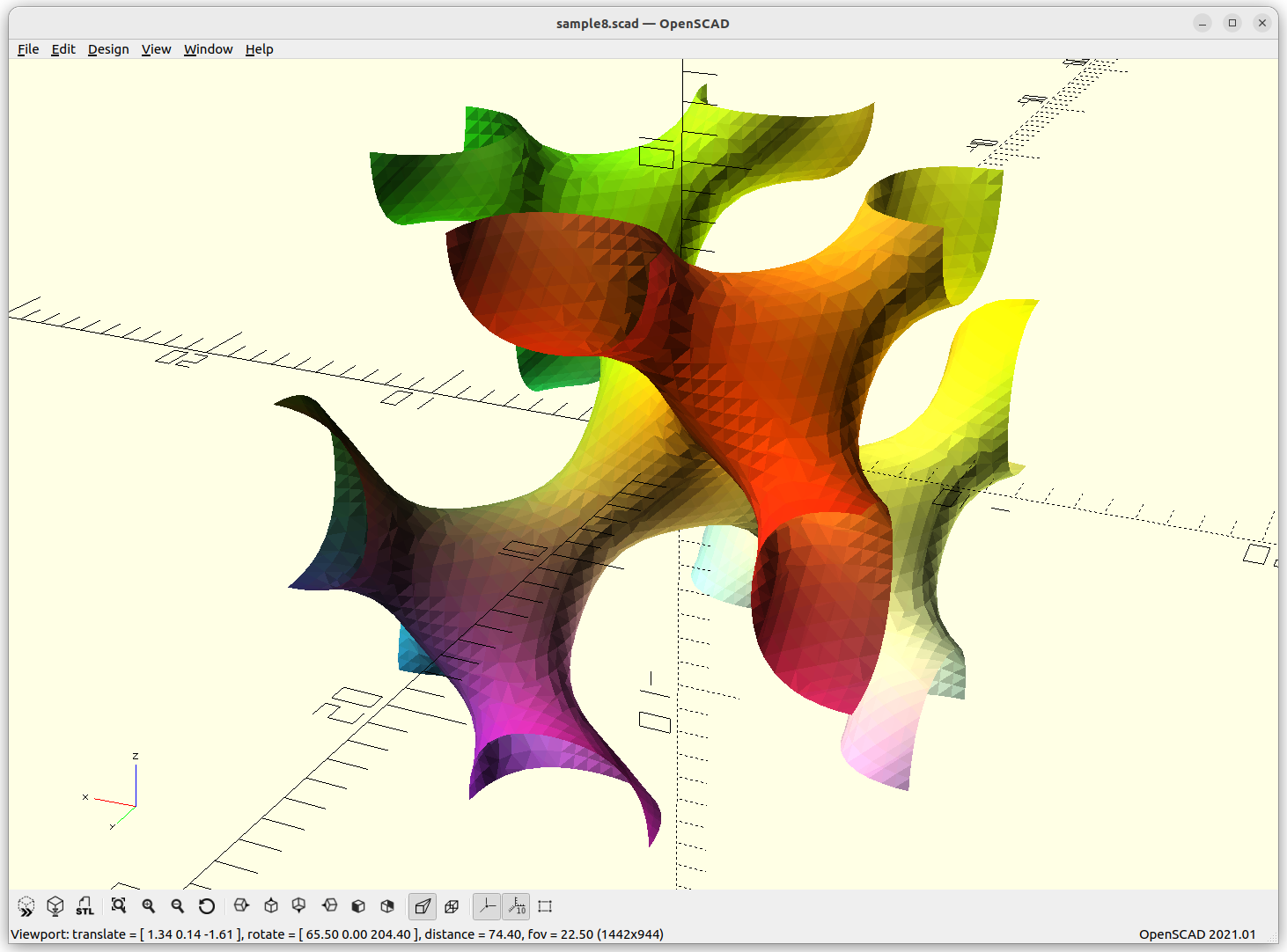

providing a structure using 4 arms to connect each other.
Miscellaneous


Using Implicit Geometries as Infill Structures
Slic3r and Prusa Slicer are providing gyroid infill pattern since early version, but beyond that it seems no to little development happened since (2022/12).
Let’s see how implicit geometry can be transformed into slices (FDM) or voxels/pixels (SLA, SLS etc)
Algorithm A: 3D Cache
- create point cloud of surface of implicit geometry
- create surface of implicit geometry using marching cube
- (optional) determine x, y, z size where it repeats itself
- slice surface for infills at certain scale
- clip inner surface with outer perimeter of slice
Pros
- with caching: fast lookup of infill geometry
Cons
- many steps
- x, y, z repeatability must be given, hard to determine programmatically from outside
- clipping to perimeter can be computational expensive depending
Algorithm B: 2D Cache
- create 2D point cloud of a slice of implicit geometry based on clipped 2D area / slice
- convert 2D point cloud to polylines (FDM) or pixels (SLA)
Pros
- reduction to 2D problem at first stage
- fast 2D point cloud creation as only one z-level is used
Cons
- create 2D point cloud at arbitrary resolution, loss of curves unless refitted
- caching without knowing repeatability of the geometry makes little sense
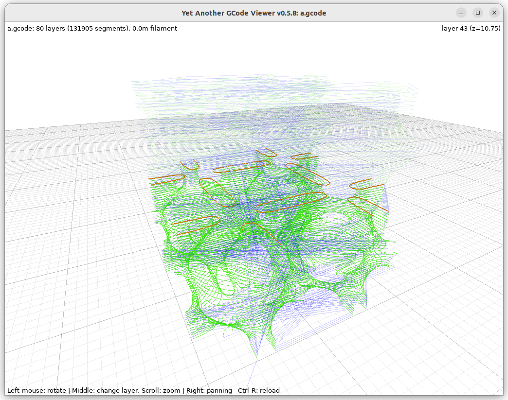
FDM G-code
Here some early G-code for FDM 3D printer using PyImplicit tool tracking the implicit surface as 2D contour:
Meshs & Voxels
The implicit surfaces only define the surface, either:
- inside vs outside – a solid; or
- certain thickness of such surface
In order to create watertight meshs the volume needs to be limited with a boundary box, and Marching Cube is performed from outside to get proper mesh to post-process afterwards.
Now you may wonder, what’s the fuss with all those forms, why doing this complicate implicit form, why not just create a few forms as meshs right away and repeat them orderly – well, here it comes why:
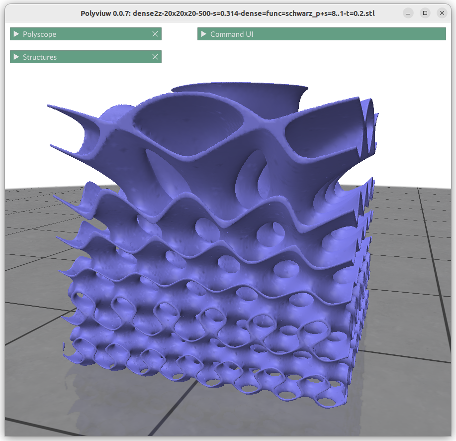
Frequency or Scale Gradients
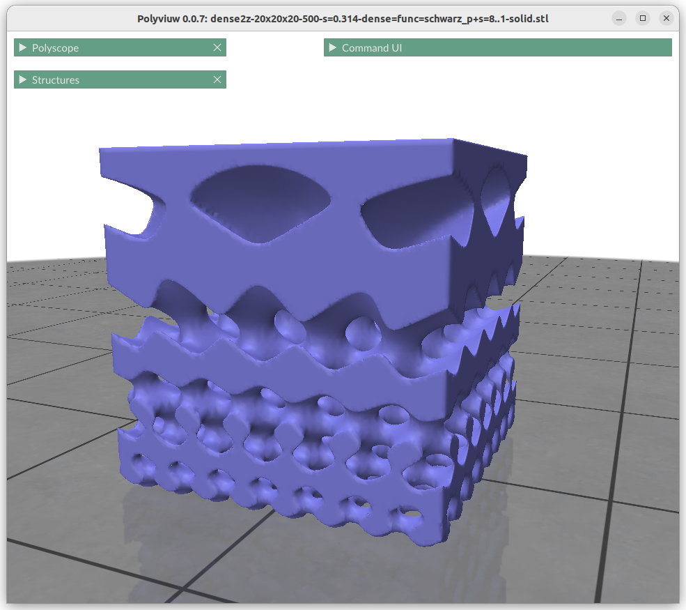

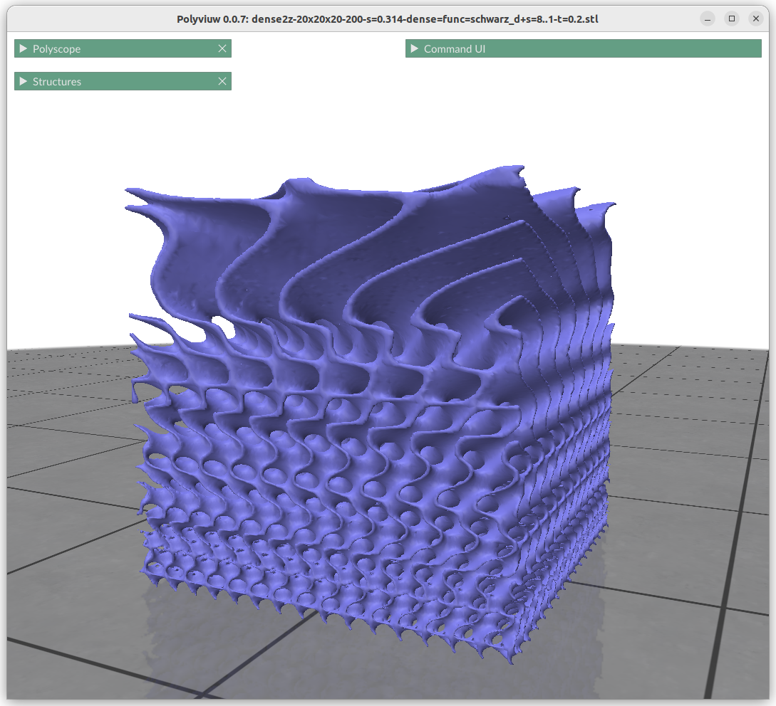
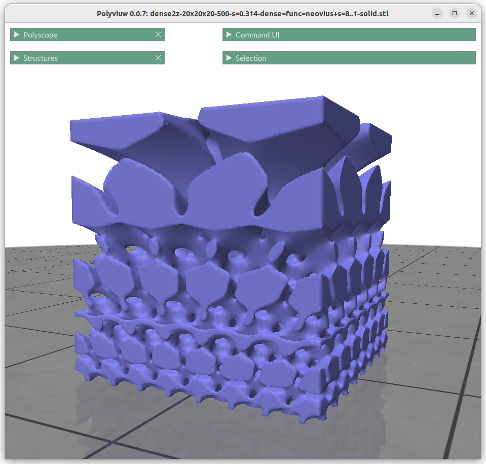
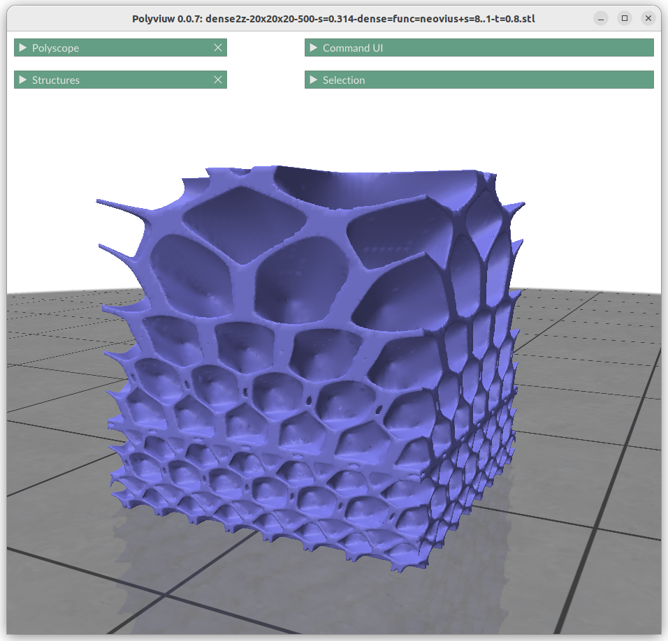
Changing the frequency or scale s0 and s1 can be achieved by:
znorm = (z-zmin) / (zmax-zmin)
s = (1-znorm)*s0 + znorm*s1 or
s = lerp(s0, s1, znorm)
f = surface(x*s, y*s, z*s)
This shows the power of generative geometries, we simply can define the scale or frequency of a geometry at any point, given we transit within reason and not too sharply to cause discontinuty.
Thickness Gardients
Alike changing thickness:
znorm = (z-zmin) / (zmax-zmin)
t = lerp(t0, t1, znorm)
f = abs(surface(x,y,z)) – t
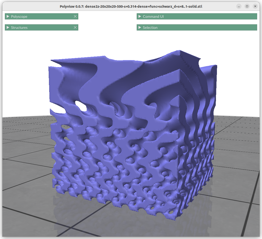
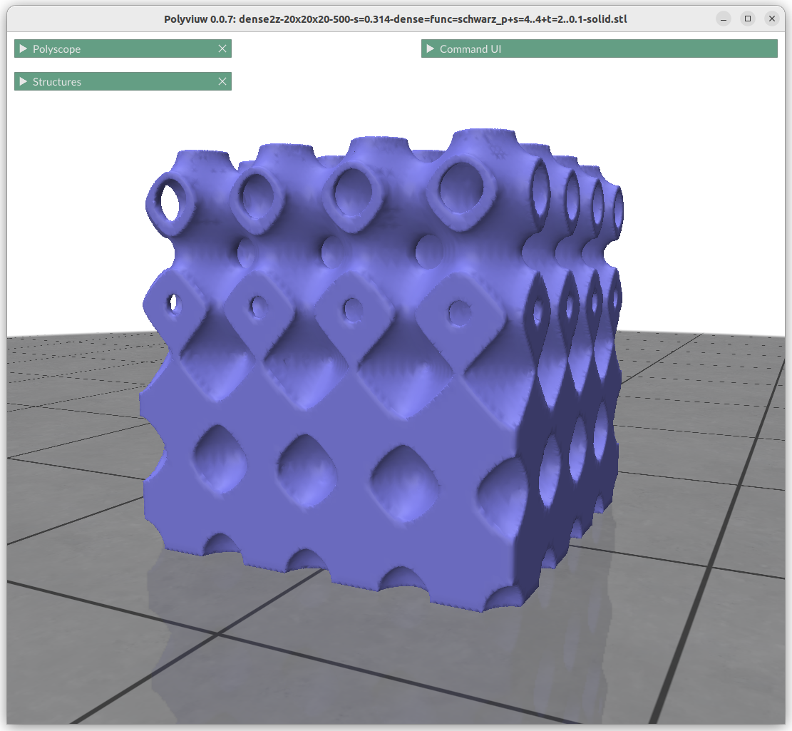
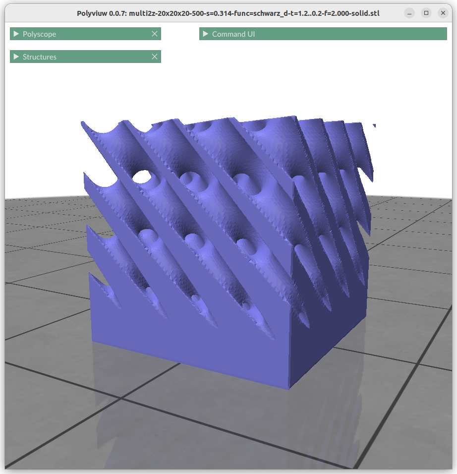
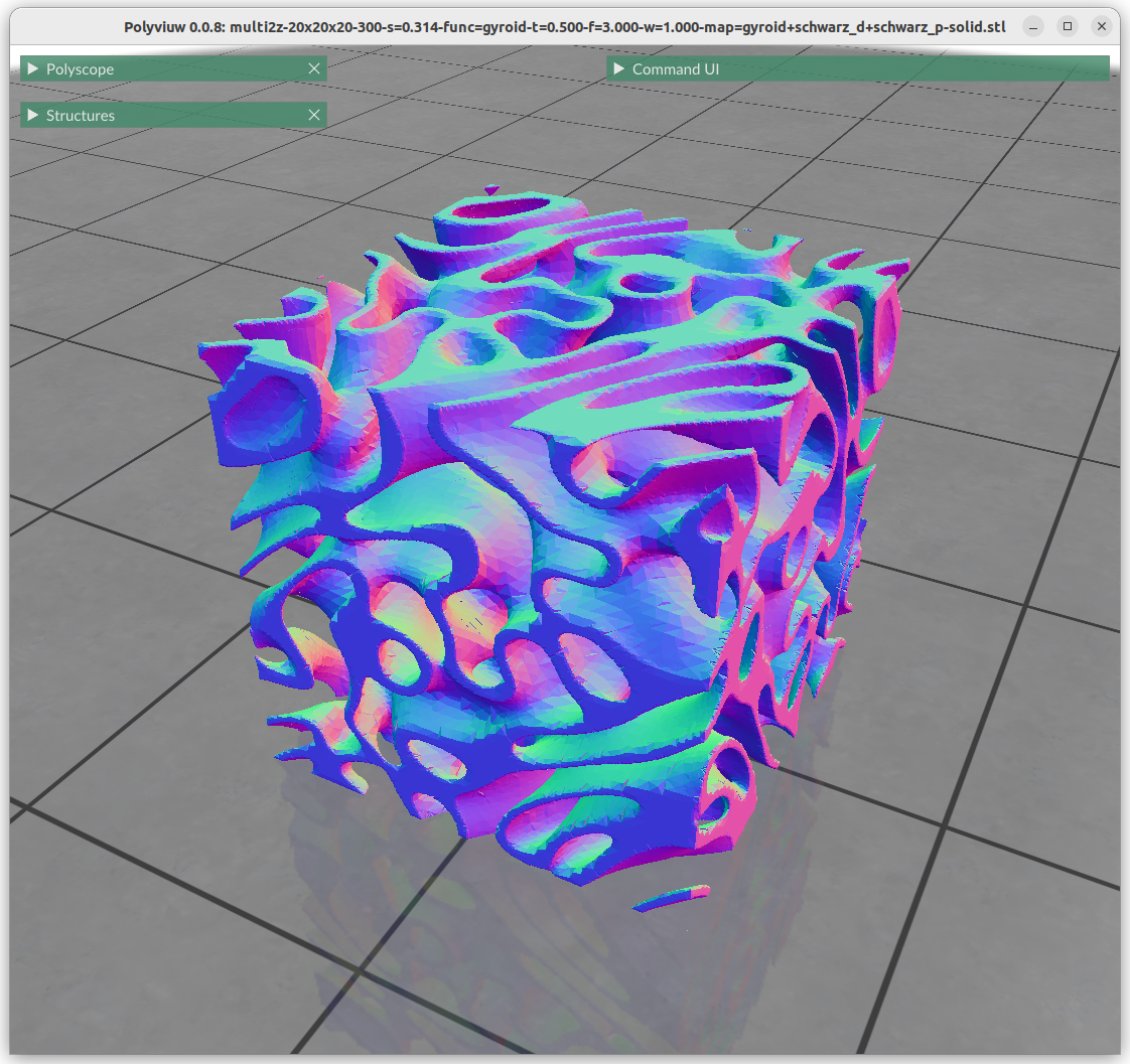
Form Gradients
What looks very complex is done quite simply with:
znorm = (z-zmin) / (zmax-zmin)
f = lerp(surface1(x,y,z) , surface2(x,y,z), znorm)
This is quite powerful property, to be able to morph from one implicit form to another with such a simple formula.
Contineous Transitions:
- Schwarz D – Schwarz P
- Schwarz D – Neovius
- Schwarz P – Neovius
- thickness: IWP Skeletal – Schwarz P
- thickness: IWP Skeletal – Schwarz D
Discontinueous Transitions:
- IWP Skeletal – P Skeletal
- IWP Skeletal – Neovius
- solid: IWP Skeletal – Schwarz P
- solid: IWP Skeletal – Schwarz D
Combining Implicit Surfaces
Additions
Algebraic addition has the effect of apply one geometry within another, alike recursion:
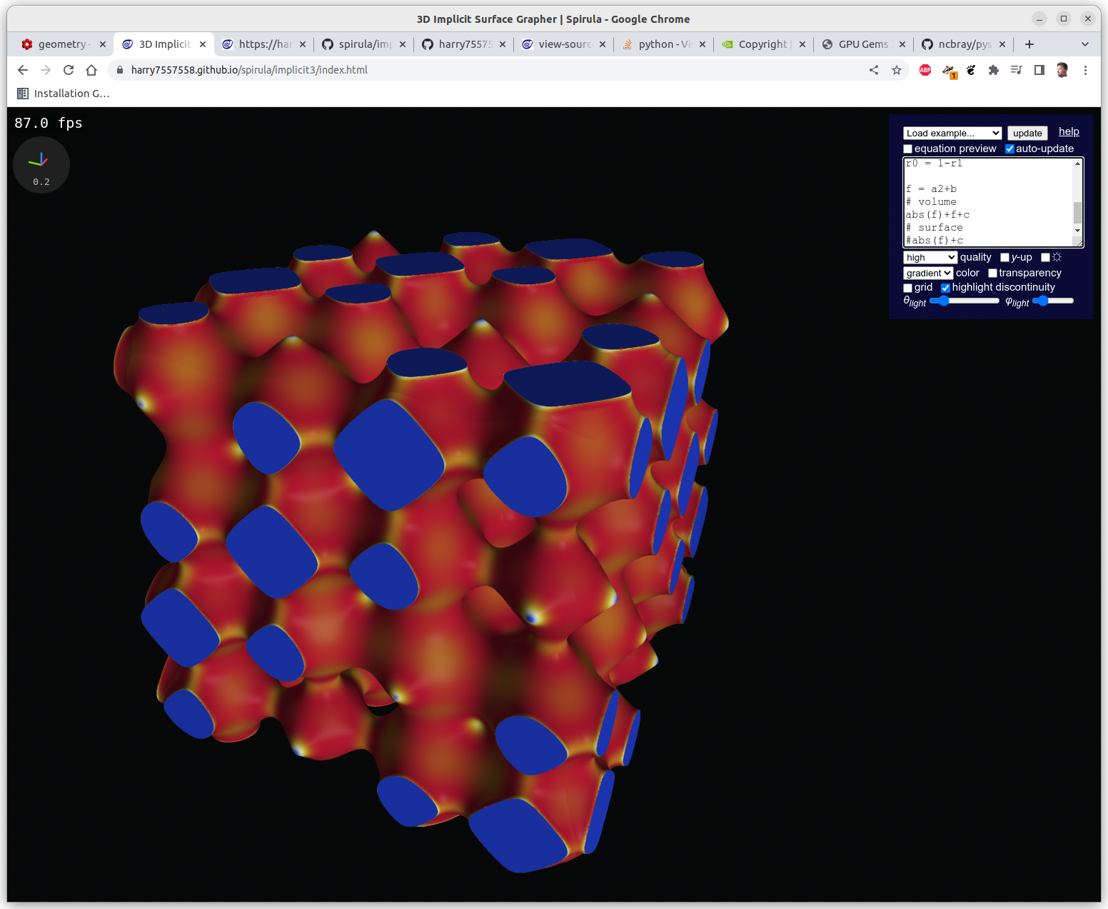
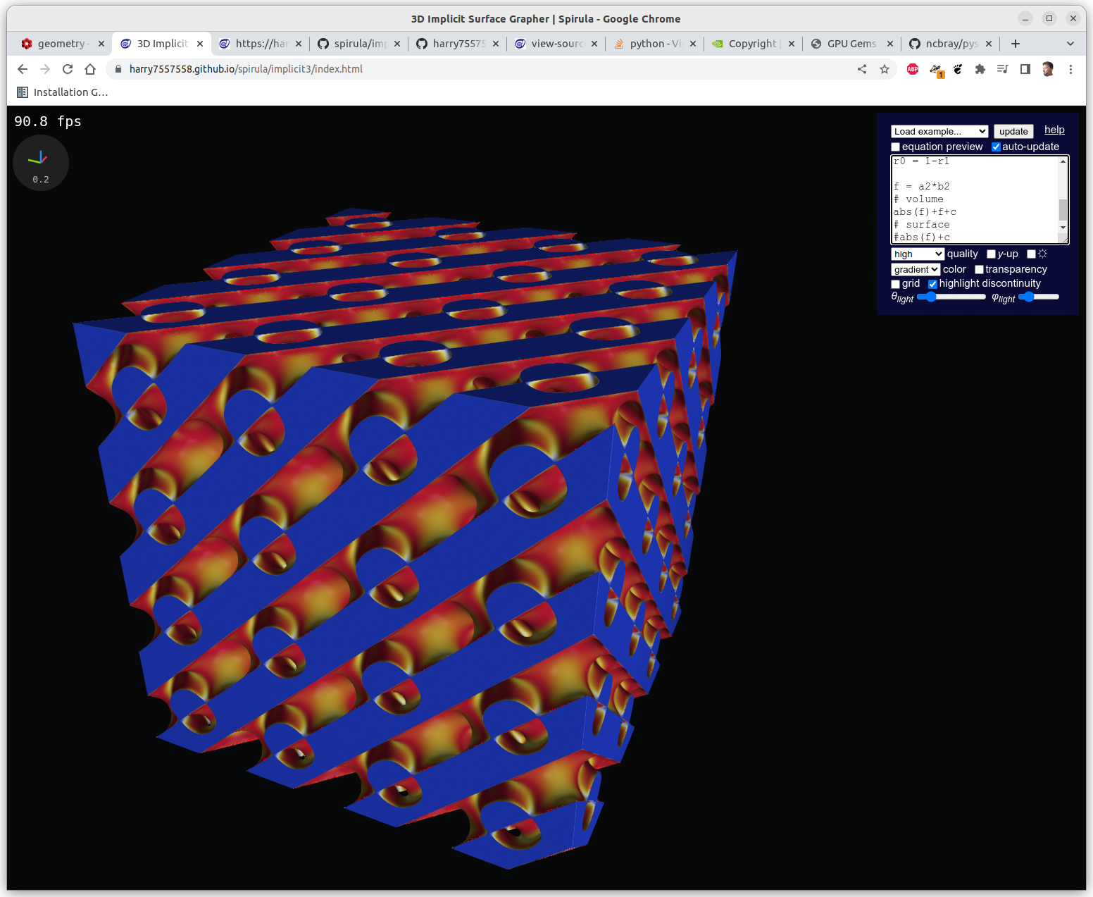
Multiplications
Algebraic multiplication has the effect of clipping, or geometrical intersection:

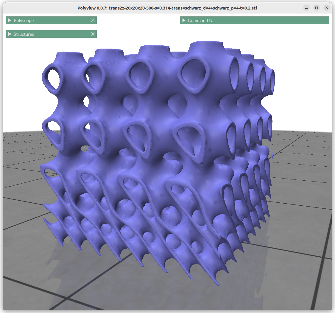
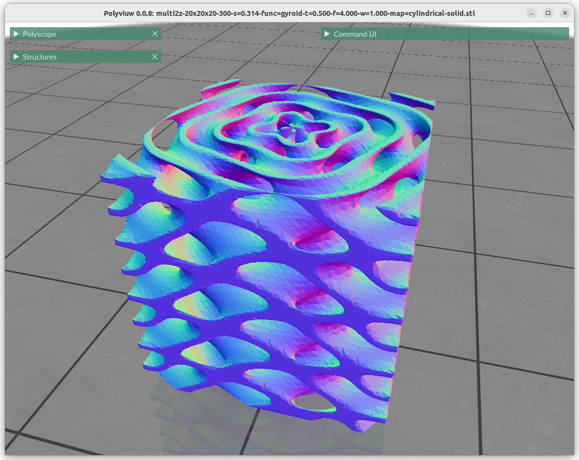
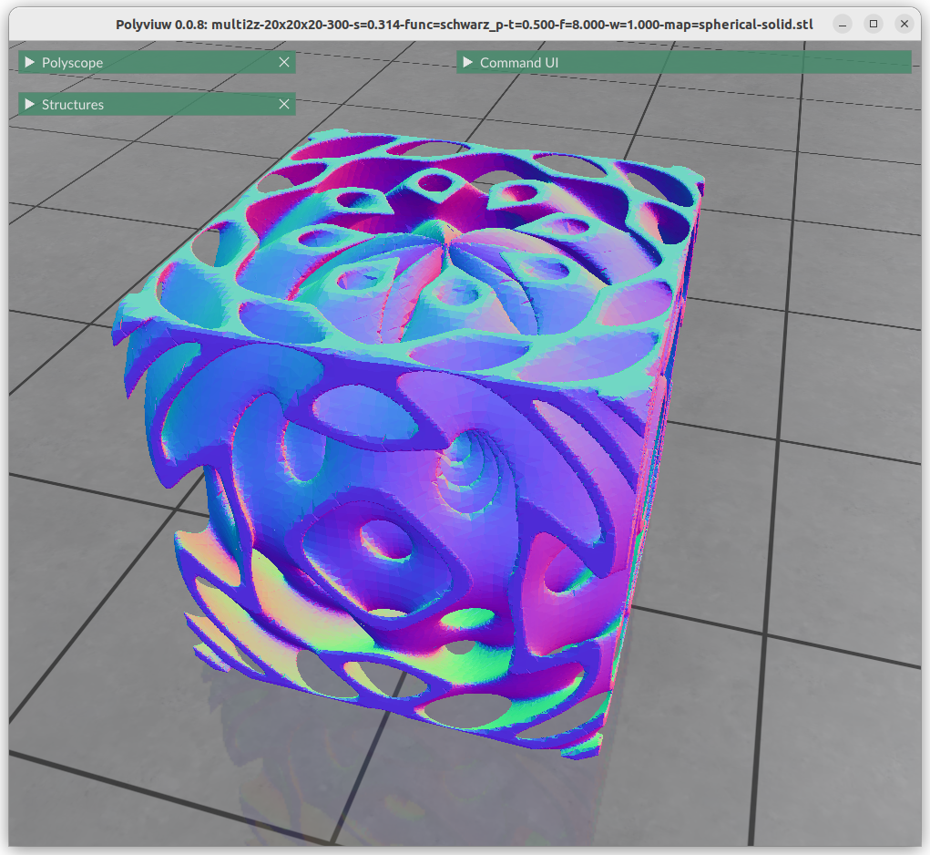
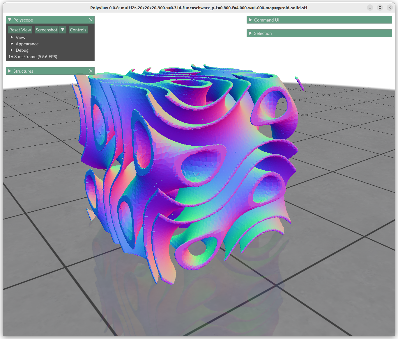
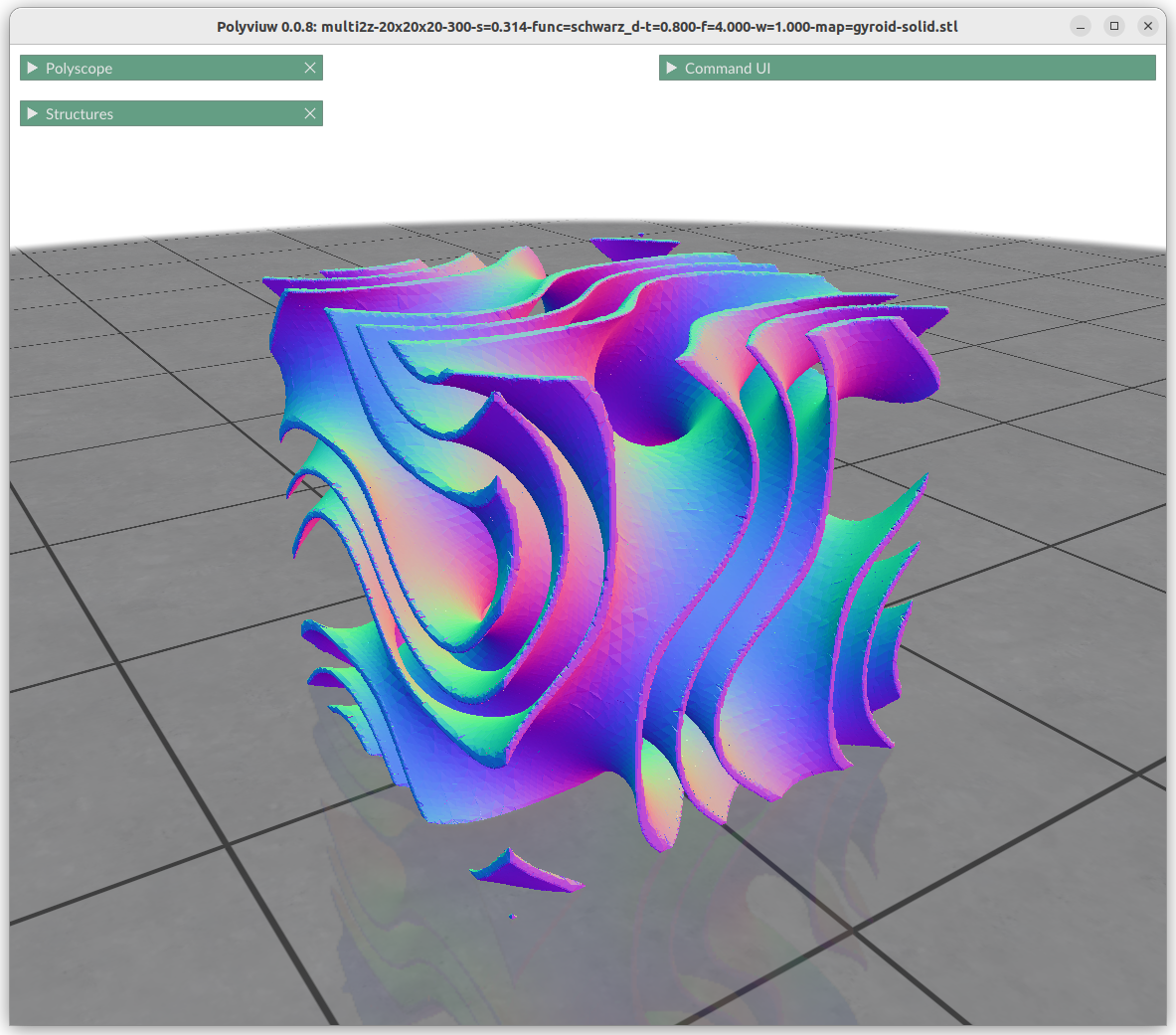
Mapping Implicit Surfaces
One can map the coordinates, and create a cylindrical gyroid, where former X & Y become distance and rotation angle, and Z remains as is, and so spherical projection is possible as well, or even feed coordinates through implicit formula itself:


Next blog-post(s) I will go into further details utilizing TPMS in Additive Manufacturing (AM) like FDM/FFF, SLA, MSLA, SLS, MJF or SLM – each one of them have unique features and limitation for using those Parametric Generative Infill Geometries.
Appendix: Visualization
In case you wondered of the different styled visualization through this blog-post, let me show you the different approaches to discretize implicit defined surfaces.
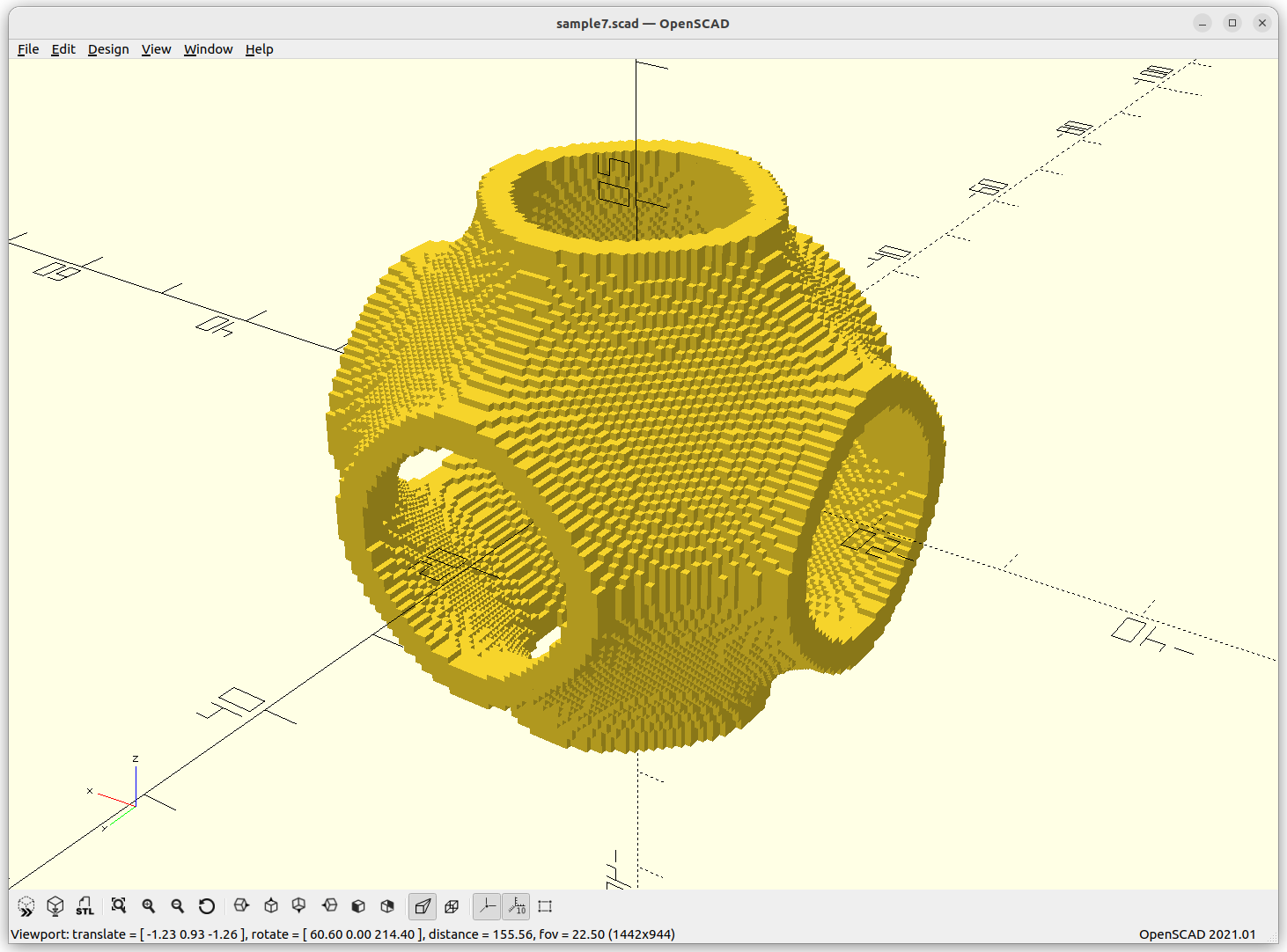
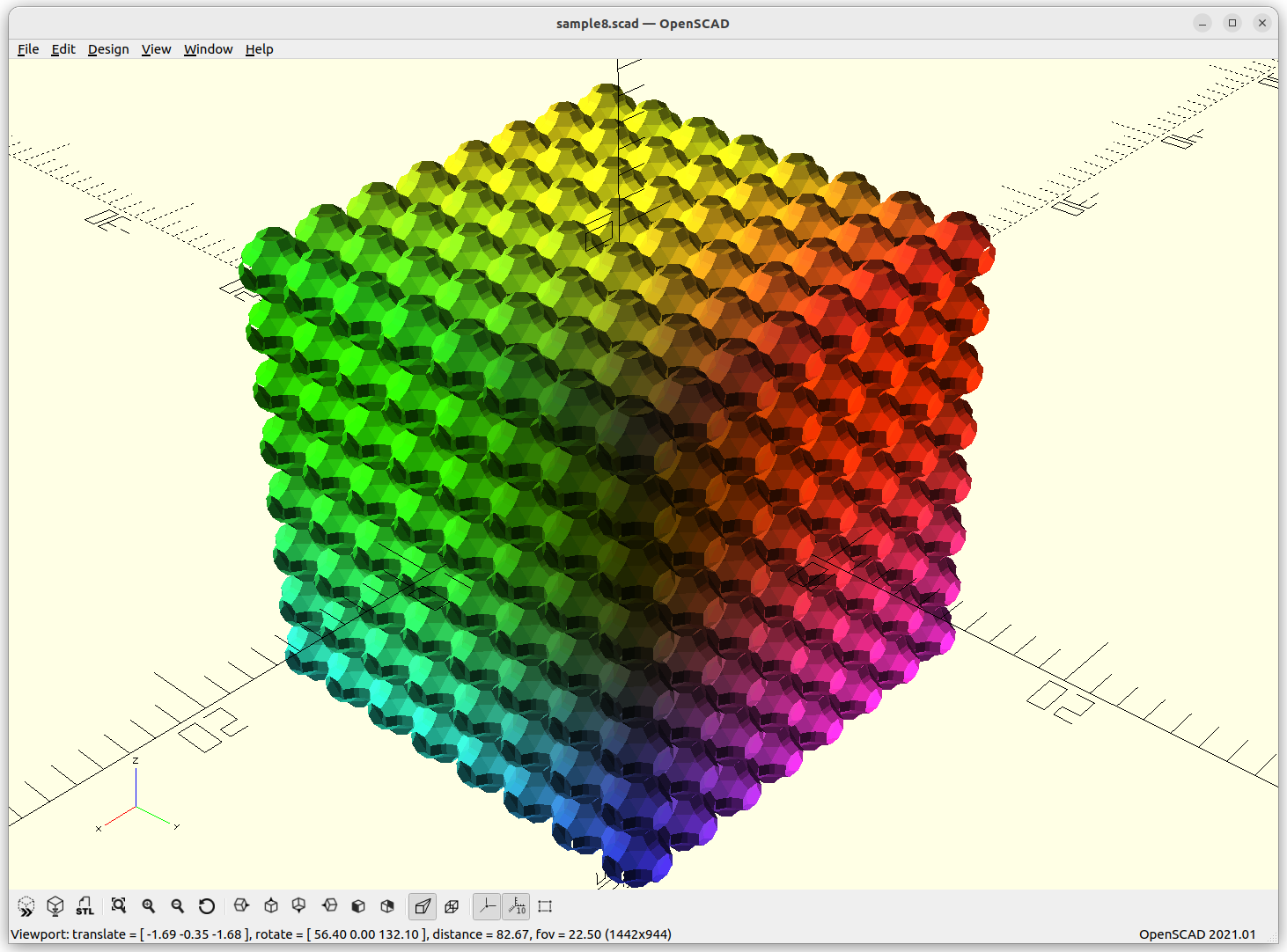
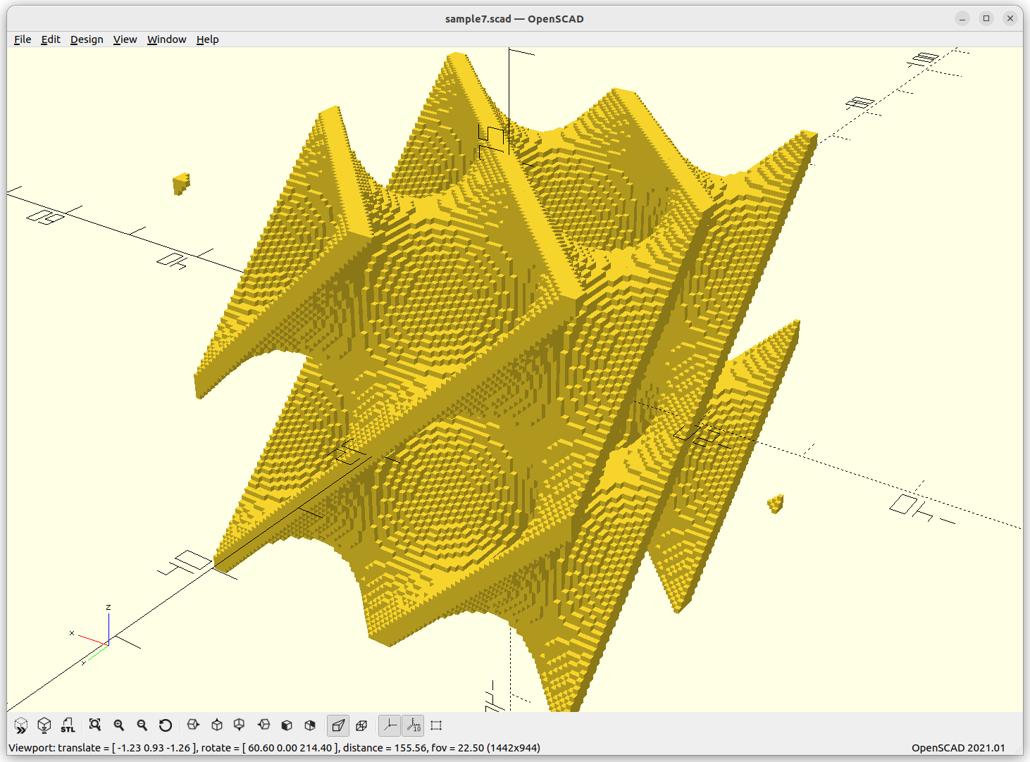
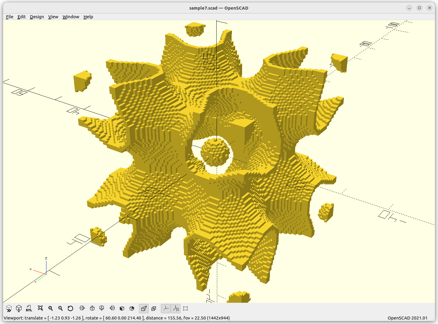
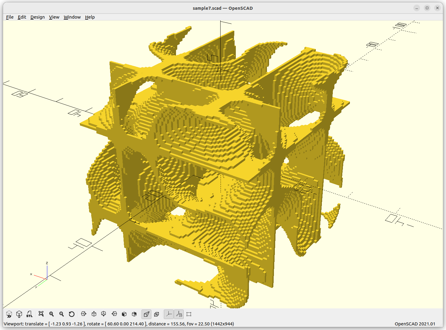
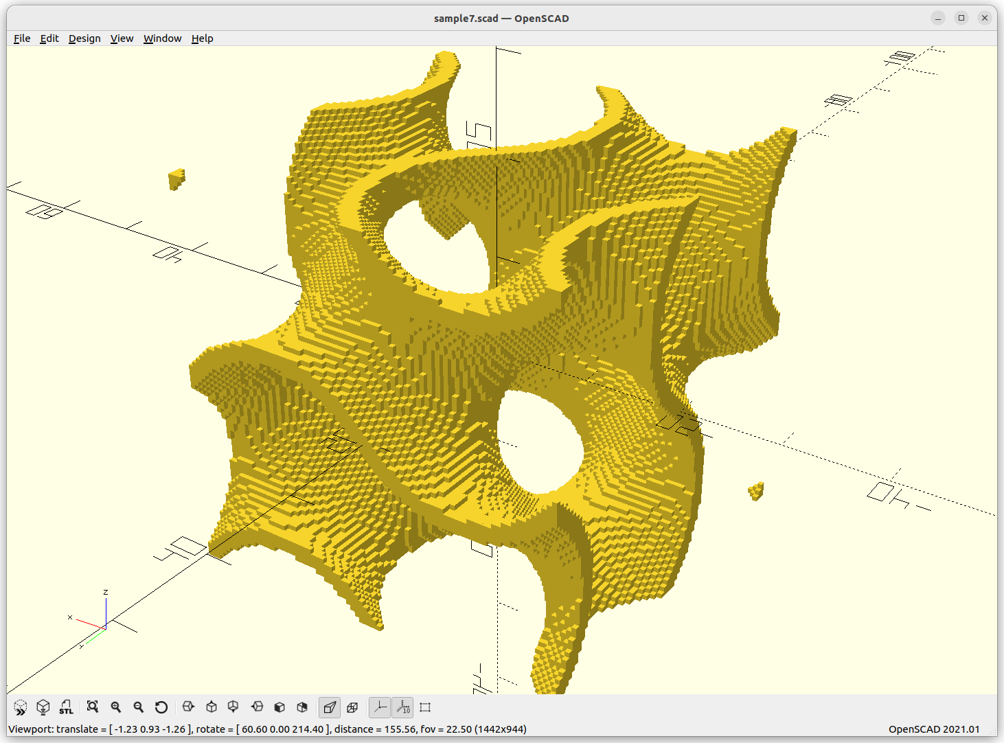
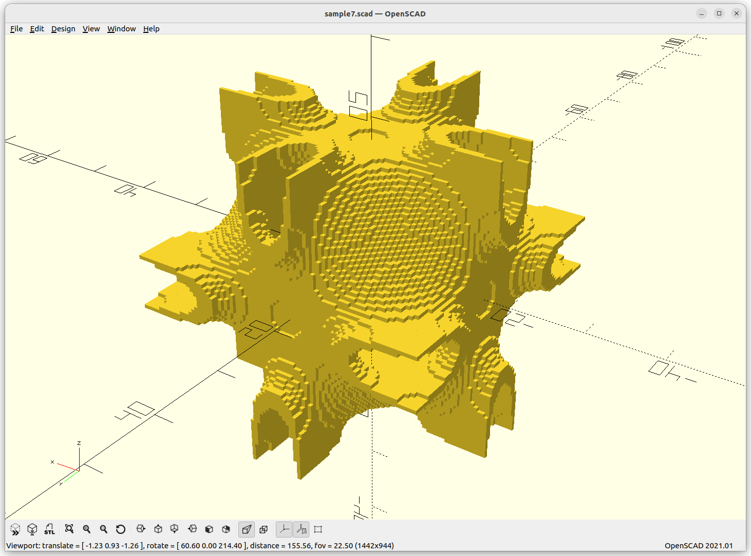
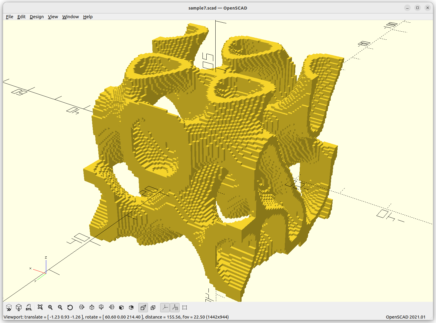
Voxels
The code is rather simple with OpenSCAD yet rather slow: either skin is true or false, and delta determines the thickness of the skin if enable:
t = 1;
r = 20*t;
st = 1/2;
delta = 0.2;

function schwarz_p(x,y,z,s=1) = cos(x*s) + cos(y*s) + cos(z*s);

skin = true;

for(x=[-r:st:r])
   for(y=[-r:st:r])
      for(z=[-r:st:r]) {
         f = schwarz_p(x,y,z,360/20/2);
         if(skin && abs(f)<delta)           // -- skin only
            translate([x,y,z]) cube(st);
         else if(!skin && f<delta)          // -- inside/outside
            translate([x,y,z]) cube(st);
      }
Rendered via voxelation:


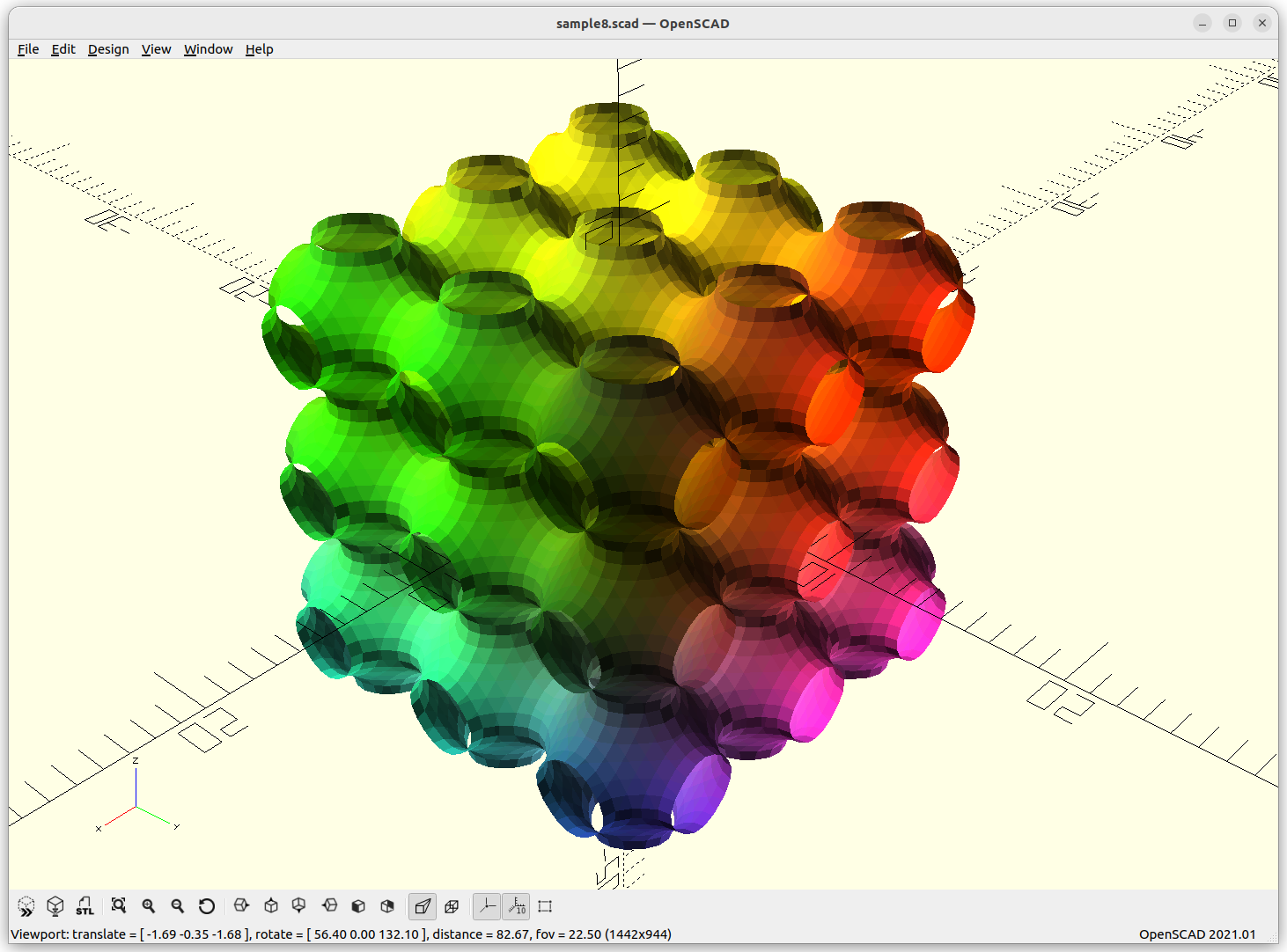
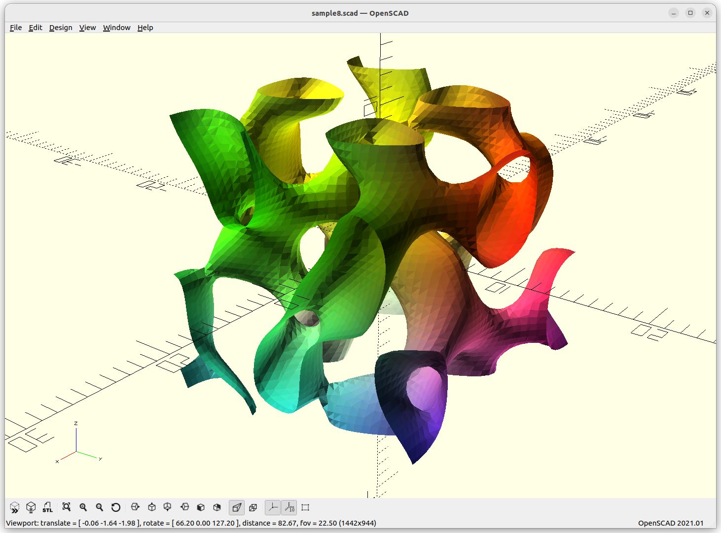
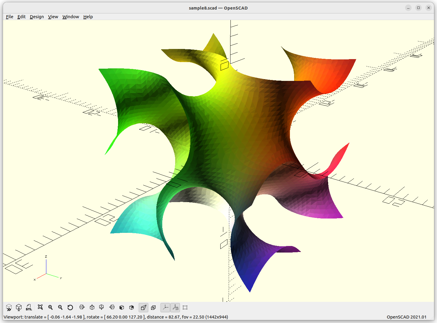
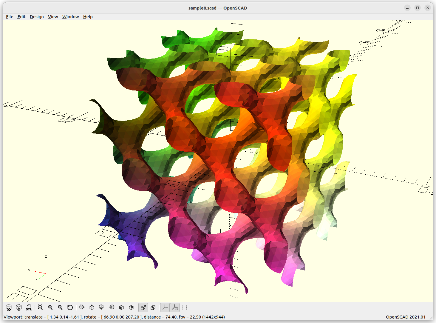
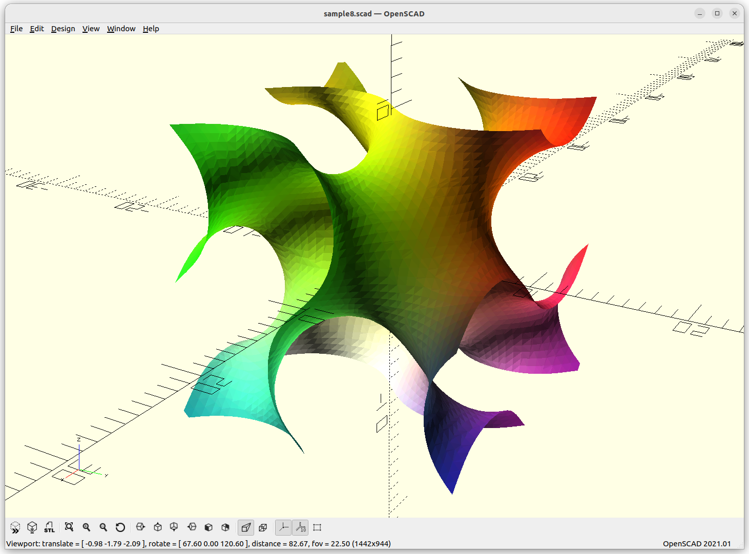
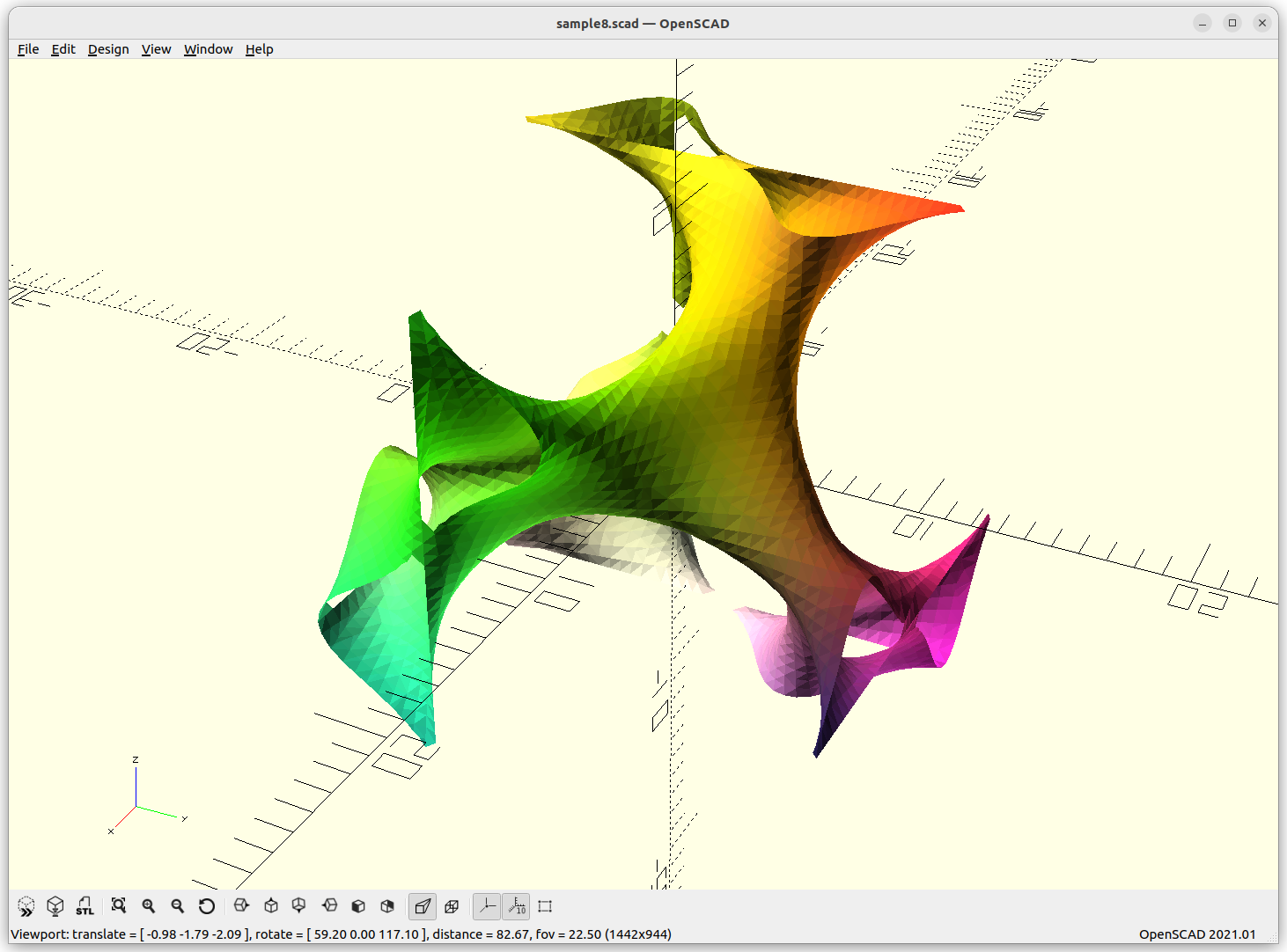
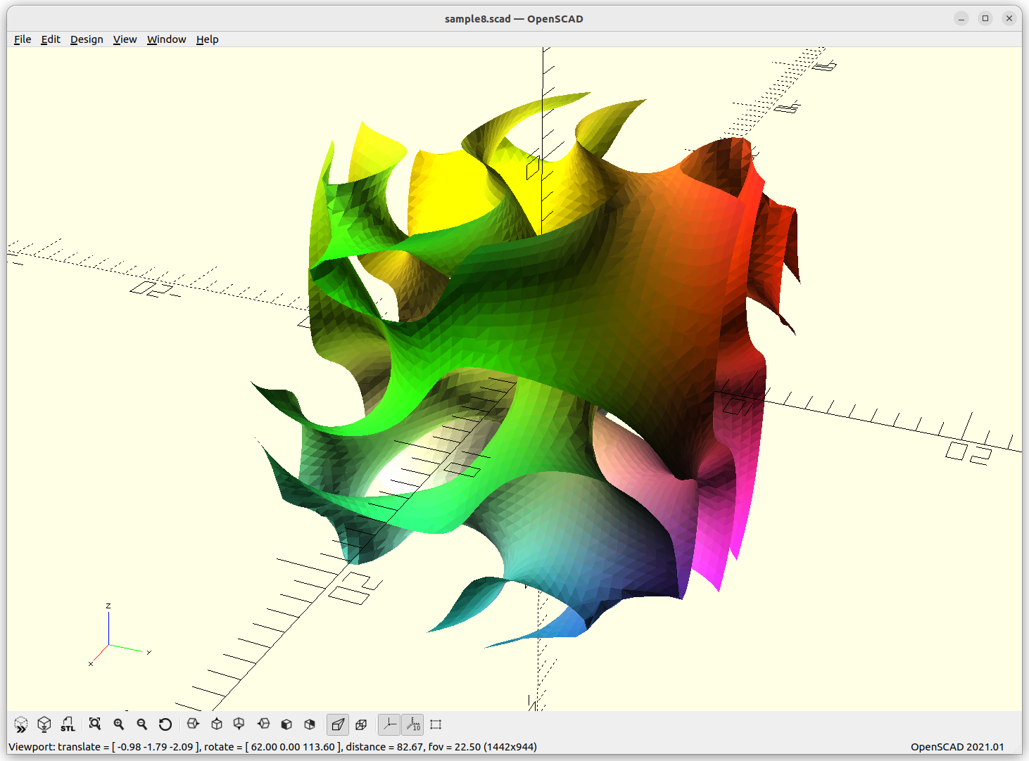
Surface
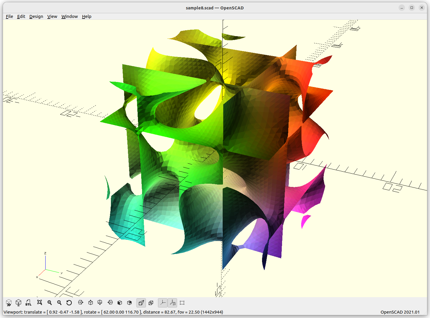
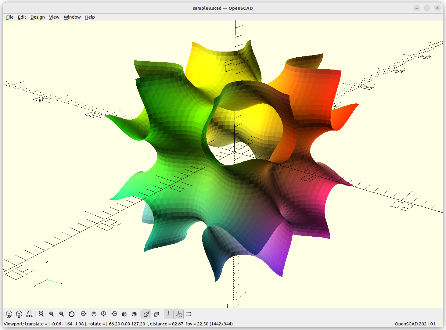
Rendered in OpenSCAD via marching cube algorithm with Level Surfaces:


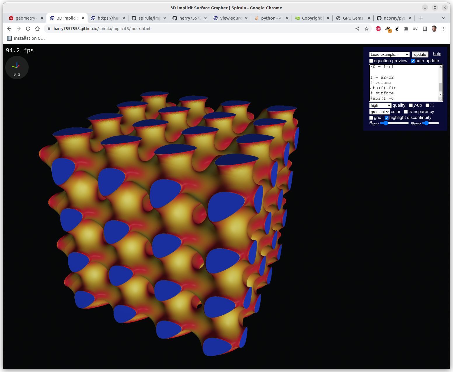
Volumes & Surfaces in OpenGL GLSL
Following experiments were done with Spirula/Implicit3 within the browser, the implicit formulas are rendered in realtime at 100-500 fps using OpenGL’s GLSL (GL Shader Language):
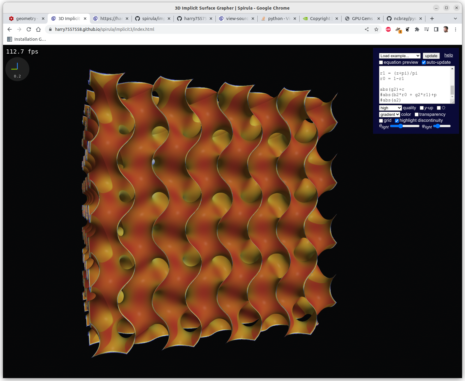

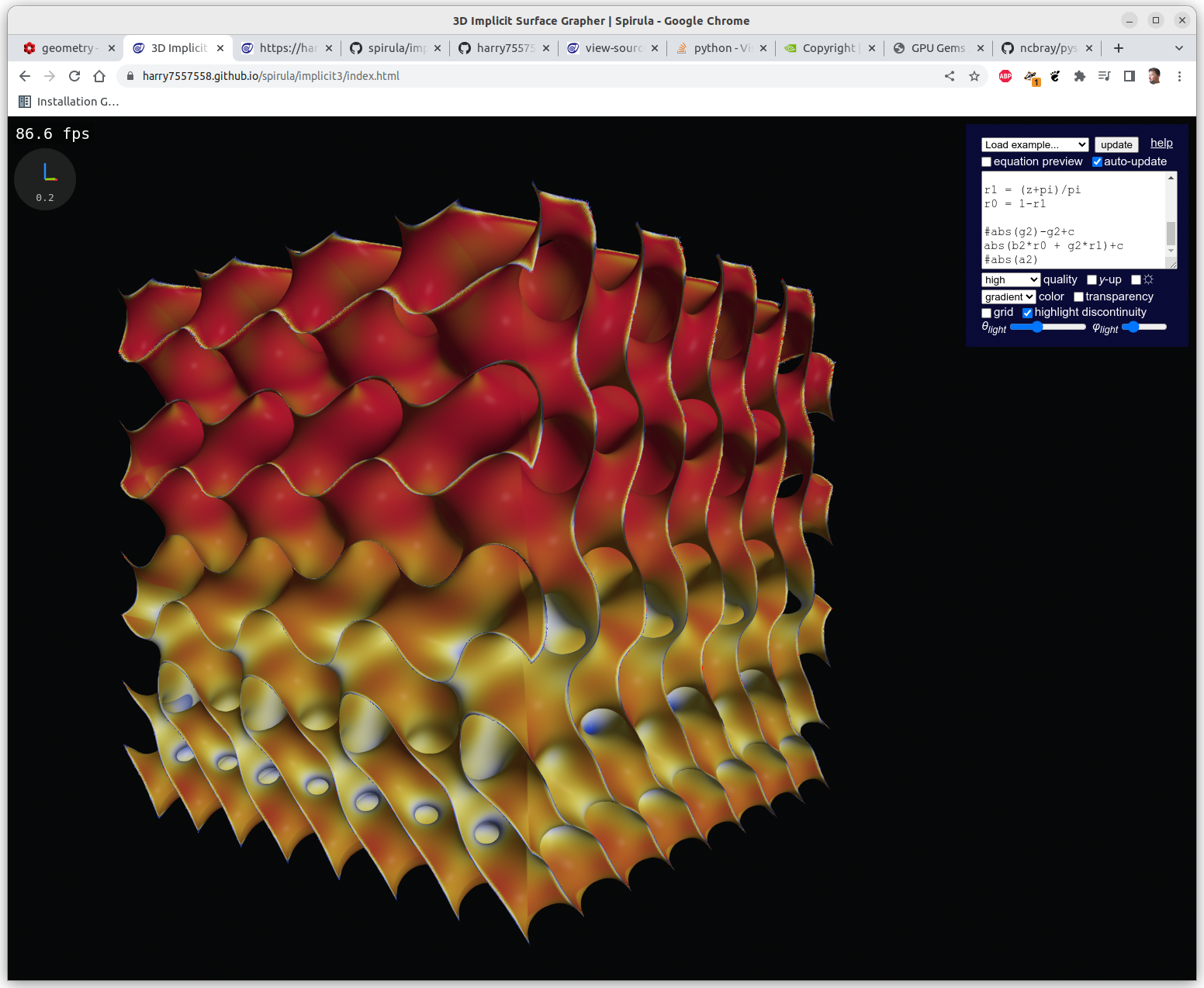
One has to clip the formulas with a cube in order to have a limited set, otherwise you get a full screen looking at infinite X, Y & Z, here Schwarz P:
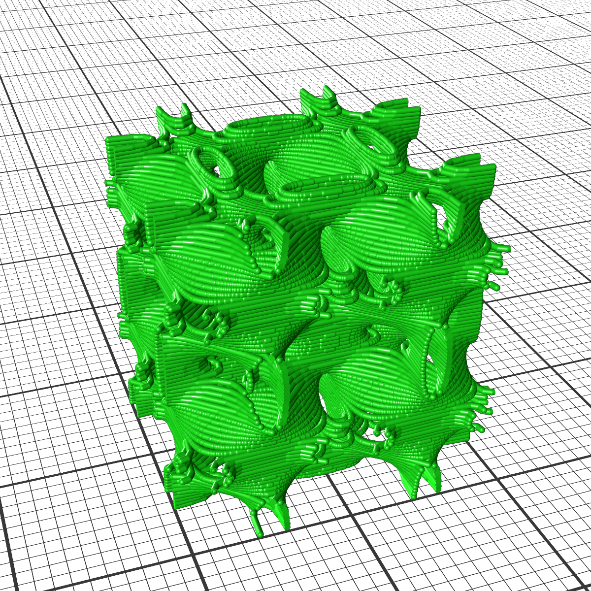
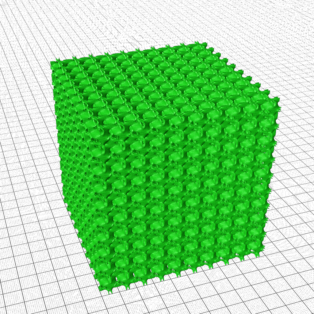
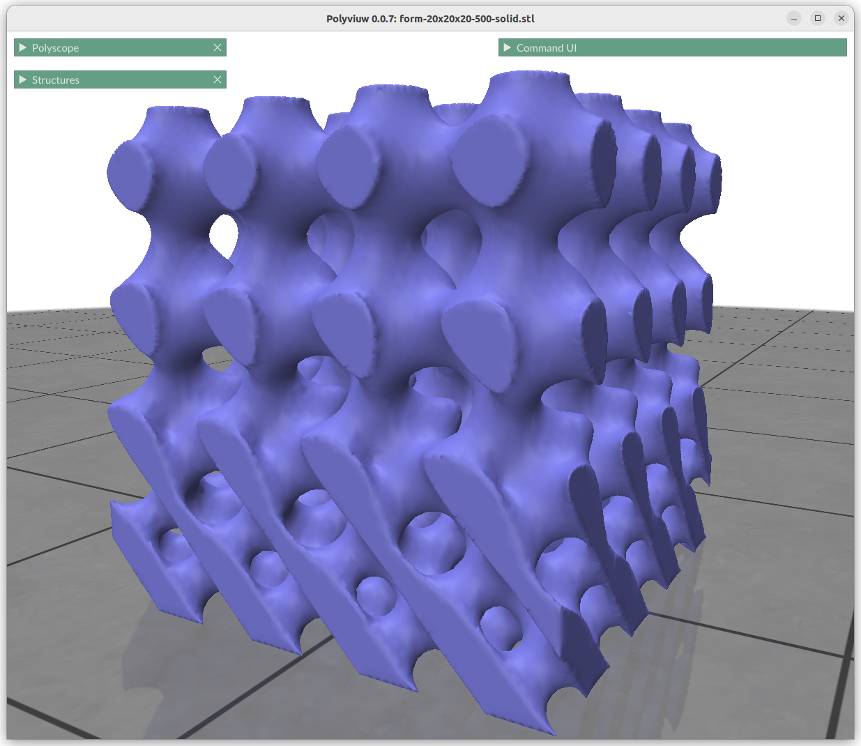
Meshs with Marching Cube
In order to create a mesh, I developed PyImplicit which utilizes Numpy library to calculate the implicit formula fast, and then run a Marching Cube algorithm over the result in order to get a discrete mesh like STL, OBJ, or 3MF to process further for 3D printing.

surface gradient between Schwarz D to Schwarz P (top) at certain thickness or solid,
2nd row: 2x IWP skeletal 90mm cubes at different frequency;
Background: various 30/40mm cube clipped Triply Periodic Minimal Surfaces
*) some of my larger prints I attach RFID tags, e.g. as on top of the variable frequency Schwarz P print, which I store the print UID from my Prynt3r job which logs all my prints with all settings and webcam snapshots. In future blog-post I will illustrate my NFC/RFID setup.
And Polyviuw is a small mesh viewer using Polyscope Python as backend to display it as mesh:
It is easy to create huge files when exporting an implicit generative infill geometry and one ends up with a 700MB binary STL file, which becomes hard to view at least on my system. To handle complex outer forms, with complex inner geometries I estimate reaching multiple gigabytes large files – let’s see.
References
- 3D-Meier.de: Juergen Meier’s excellent write-up on Triply Periodic Minimal Surfaces (german only) with formulas & references
- Commercial Software:
- nTopology.com: outer and inner geometry incl. simulation
- GeoDict.com: digital material development, deep dive into designing interior geometries
- Spherene.ch: Adaptive Density Minimal Surfaces (ADMS) software framework, startup
- Metafold3D.com: volumetric design, combining interior (infill) and exterior structures (mesh boundaries); cloud API, startup
- Papers:
- [Panesar, Abdi, Hickmann, Ashcroft] Strategies for functionally graded lattice structures derived using topology optimisation for Additive Manufacturing (PDF)
- [Singh, Narayanan] Real-Time Ray-Tracing of Implicit Surfaces on the
GPU (PDF) - [Feng, Fu, Yao, He] Triply periodic minimal surface (TPMS) porous structures (PDF)
- [Ntintakis, Stavroulakis] Infill Microstructures for Additive Manufacturing (PDF)
- and many more
- Github:
- Level Surfaces: OpenSCAD based 3D surface grapher (OpenSCAD)
- Spirula (WebGL), instant preview of implicit surfaces in browser using GPU
- PyMCubes, marching cubes
- Scaffolder, Python / Blender plugin mixing meshs with TPMS
- Miscellaneous:
- From Triply Periodic Minimal Surface to Architecture by Catherine Zhang
- Inigo Quilez: Distance Functions, the jewels of SDFs / implicit formula